Computer Vision Explained: Tasks, Models, and Applications

Computer vision is the field of AI that teaches machines to extract meaning from images and video: what is in a picture, where it is, and what is happening. If you have ever unlocked a phone with your face, scanned a document into text, or watched a car hold its lane, you have used it.

This guide explains computer vision from the ground up. You will learn how images become numbers, the four core tasks (classification, detection, segmentation, and tracking), the main model families from convolutional neural networks to Vision Transformers, how to evaluate results, and how to run two real models in Python. It also covers where computer vision connects to generative AI, and where it still fails.

What Is Computer Vision?

Computer vision (CV) is a branch of artificial intelligence and machine learning that builds systems able to interpret visual data. The input is an image or a video. The output is something useful: a label, a set of boxes, a mask, a measurement, or a text description.

It is hard because a computer does not see objects. It receives a grid of numbers, and it has to learn which patterns in those numbers correspond to “cat”, “crack in a pipe”, or “pedestrian”. The same object can appear under different lighting, angles, sizes, and partial occlusion, so the model must learn what stays constant.

How a Computer Sees an Image

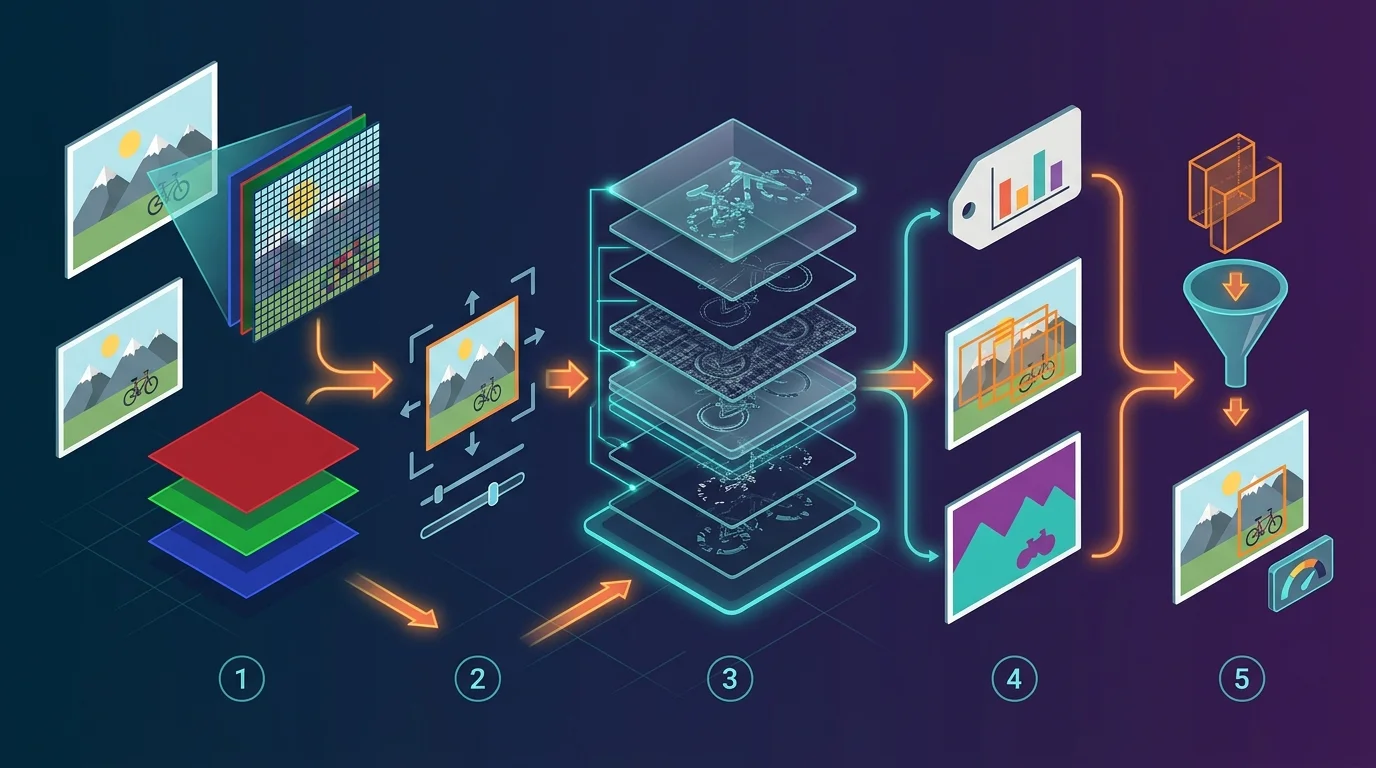
A grayscale image is a 2D grid of pixels, each holding a brightness value, commonly 0 (black) to 255 (white). A colour image adds a third dimension: three channels (red, green, blue), so a photo of 224 by 224 pixels is stored as a 224 × 224 × 3 array of numbers.

Everything in computer vision starts from that array. Classical methods applied hand-designed filters to find edges and corners. Modern deep learning learns its own filters from data.

A worked example: finding an edge with convolution

The core operation behind CNNs is the convolution. You slide a small grid of weights, called a kernel, across the image. At each position you multiply the kernel by the pixels underneath and add the results:

$$\text{out}(i,j) = \sum_{m}\sum_{n} I(i+m,\, j+n)\; K(m,n)$$

Here $I$ is the image, $K$ is the kernel, and $(i,j)$ is the position of the window. (Deep learning libraries technically compute cross-correlation, but the name “convolution” stuck.)

Below is a tiny image that is dark on the left and bright on the right, and a Sobel kernel that responds to vertical edges.

import numpy as np

# 6x6 grayscale "image": dark left half (0), bright right half (9)
image = np.array([[0, 0, 0, 9, 9, 9]] * 6, dtype=float)

# Sobel kernel that responds to vertical edges (left-to-right brightness change)
kernel = np.array([[-1, 0, 1],
                   [-2, 0, 2],
                   [-1, 0, 1]], dtype=float)

def convolve2d(img, k):
    kh, kw = k.shape
    out_h, out_w = img.shape[0] - kh + 1, img.shape[1] - kw + 1
    out = np.zeros((out_h, out_w))
    for i in range(out_h):
        for j in range(out_w):
            out[i, j] = np.sum(img[i:i + kh, j:j + kw] * k)
    return out

print(convolve2d(image, kernel))

Output:

[[ 0. 36. 36.  0.]
 [ 0. 36. 36.  0.]
 [ 0. 36. 36.  0.]
 [ 0. 36. 36.  0.]]

The two middle columns light up with 36 exactly where brightness jumps from 0 to 9; flat regions give 0. A CNN does the same thing, except it learns hundreds of kernels automatically, and stacks layers so that early layers detect edges, middle layers detect textures and parts, and deeper layers detect whole objects.

The Core Computer Vision Tasks

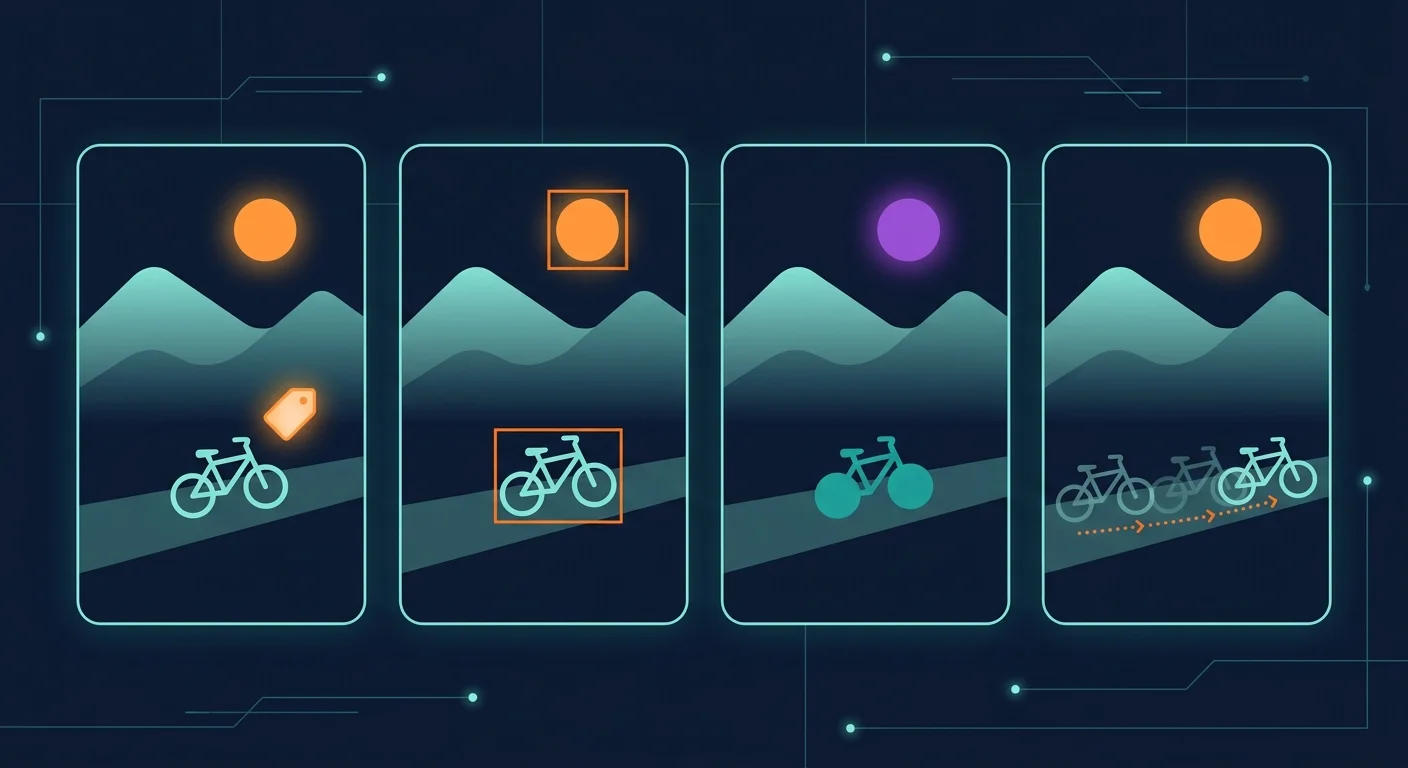
Most applications are built from a small set of tasks. Knowing which one you need is the most useful decision you will make, because it determines the model, the data labels, and the metric.

1- Image classification

Classification assigns one label (or a few) to a whole image: “this X-ray is normal”, “this photo shows a dog”. It is the simplest task and the usual starting point for learning. Its limitation is that it says nothing about where things are or how many there are.

2- Object detection

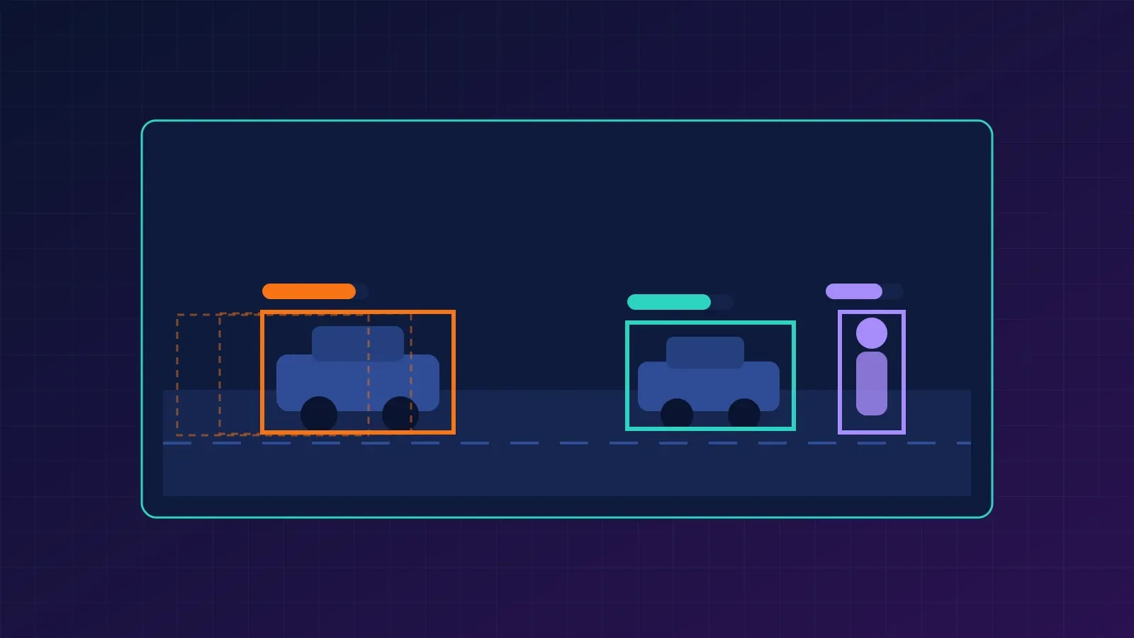
Object detection finds each object and returns a bounding box plus a class label and confidence score. It answers “what is here and where?” It is the workhorse of retail analytics, driver assistance, and security systems.

Detectors are judged with Intersection over Union (IoU), the overlap between a predicted box and the ground-truth box:

$$\text{IoU} = \frac{\text{area of overlap}}{\text{area of union}}$$

An IoU of 1 is a perfect match and 0 means no overlap. A prediction usually counts as correct when IoU passes a threshold such as 0.5, and the headline metric, mean Average Precision (mAP), averages precision across classes and thresholds.

3- Image segmentation

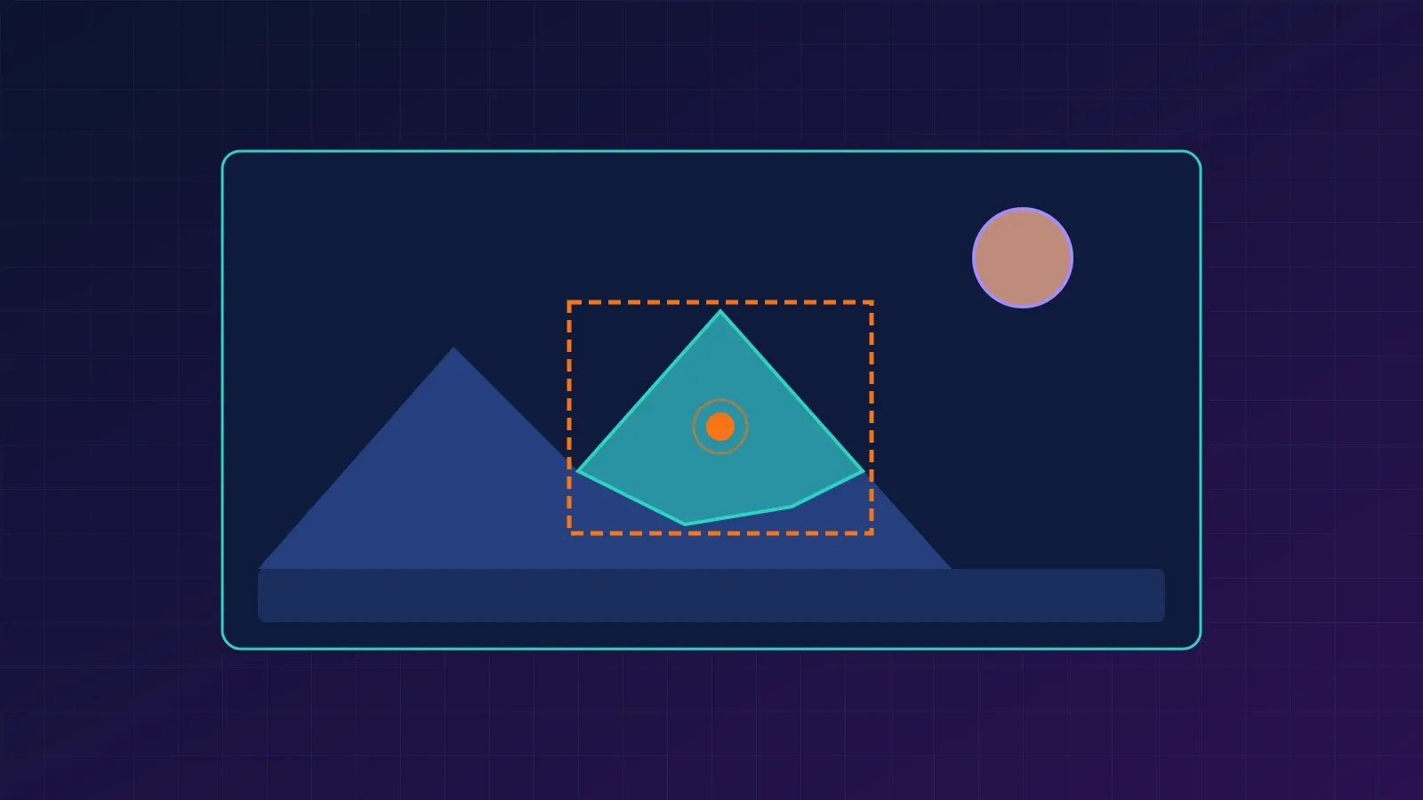
Segmentation labels at the pixel level, giving exact shapes rather than rough boxes. It comes in three flavours:

• Semantic segmentation: every pixel gets a class (road, sky, person), but two people are not distinguished.
• Instance segmentation: each individual object gets its own mask.
• Panoptic segmentation: combines both, labelling background “stuff” and individual “things”.

Use it when shape matters: tumour boundaries in medical scans, field boundaries in satellite images, or cutting a subject out of a photo.

4- Tracking, video, and other tasks

Video adds time. Object tracking keeps the same identity on an object across frames, and action recognition classifies what is happening over a clip. Other common tasks include pose estimation (locating body joints), optical character recognition (OCR) for reading text, depth estimation, and image captioning, which links vision to language.

Computer Vision Models: From CNNs to Vision Transformers

The tasks above are solved by a handful of architecture families. Many modern systems combine them: a backbone that turns pixels into features, plus a task-specific head.

1- Convolutional neural networks (CNNs)

CNNs apply learned kernels with shared weights, which makes them efficient and good at local patterns. AlexNet’s success in the 2012 ImageNet competition kicked off the deep learning era in vision, and ResNet (2015) introduced skip connections that made very deep networks trainable. CNNs remain a strong, efficient default, especially with limited data or compute.

2- Vision Transformers (ViT)

The Vision Transformer splits an image into fixed-size patches (16 × 16 pixels in the original paper), treats each patch like a word token, and applies a Transformer. With enough training data and pretraining, ViTs match or beat CNNs, and their design scales well. The trade-off is that they typically need more data or pretraining than a CNN to shine, since they do not have convolution’s built-in assumptions about locality.

3- Detection architectures

• Two-stage detectors such as Faster R-CNN first propose candidate regions, then classify and refine each. They are accurate but slower.
• One-stage detectors such as the YOLO family predict boxes and classes in a single pass, which suits real-time use.
• Transformer-based detectors such as DETR treat detection as set prediction and remove hand-tuned components such as anchor boxes and non-maximum suppression.

4- Segmentation architectures

U-Net is the classic encoder-decoder for pixel-level prediction and remains popular in medical imaging. Mask R-CNN extends Faster R-CNN with a mask branch for instance segmentation. Foundation models such as the Segment Anything line go further: Meta’s SAM 3, released in November 2025, can detect, segment, and track objects in images and video from text or example-image prompts, instead of needing a model trained for fixed classes.

5- Vision-language models

Models such as CLIP are trained on image-text pairs so that pictures and captions land near each other in a shared space. This enables zero-shot classification: you describe the categories in words and the model scores the image against them, with no task-specific training. Multimodal assistants build on the same idea.

Which model should you choose?

Your goal	Good starting point	Main trade-off
Classify images, small dataset	Pretrained CNN (ResNet) fine-tuned	Needs labelled examples per class
Classify with lots of data or pretraining	Vision Transformer	More compute and data hungry
Real-time detection on video	One-stage detector (YOLO-style)	Slightly lower accuracy on small objects
Highest-accuracy detection	Two-stage detector (Faster R-CNN)	Slower inference
Medical or precise pixel masks	U-Net or Mask R-CNN	Costly pixel-level annotation
Categories change often, few labels	CLIP-style zero-shot model	Less accurate than a tuned specialist
Quick masks of arbitrary objects	Promptable model (SAM family)	Heavier; output still needs review

Treat the table as a starting point, not a verdict. Always compare on your own data.

Run Two Models in Python

The examples below use PyTorch’s torchvision, whose pretrained model builders and weights.transforms() helpers are documented in the official torchvision docs.

Install the dependencies:

pip install torch torchvision pillow

Pretrained weights download automatically on first use, so you need an internet connection. Put any photo named street.jpg in the same folder.

Classify an image with ResNet-50

import torch
from PIL import Image
from torchvision.models import resnet50, ResNet50_Weights

weights = ResNet50_Weights.DEFAULT
model = resnet50(weights=weights).eval()
preprocess = weights.transforms()          # resize, crop, normalize as the model expects

img = Image.open("street.jpg").convert("RGB")
batch = preprocess(img).unsqueeze(0)       # add batch dimension

with torch.inference_mode():
    probs = model(batch).squeeze(0).softmax(0)

top5 = probs.topk(5)
for score, idx in zip(top5.values, top5.indices):
    print(f"{weights.meta['categories'][idx]:<25} {score:.1%}")

You will see five ImageNet class names with probabilities. Remember that ImageNet has 1,000 fixed classes: the model must pick from them even if your photo shows something else.

Detect objects with Faster R-CNN

import torch
from torchvision.io import read_image
from torchvision.models.detection import (
    fasterrcnn_resnet50_fpn_v2,
    FasterRCNN_ResNet50_FPN_V2_Weights,
)
from torchvision.transforms.functional import to_pil_image
from torchvision.utils import draw_bounding_boxes

weights = FasterRCNN_ResNet50_FPN_V2_Weights.DEFAULT
model = fasterrcnn_resnet50_fpn_v2(weights=weights, box_score_thresh=0.7).eval()
preprocess = weights.transforms()

img = read_image("street.jpg")             # uint8 tensor, shape (3, H, W)

with torch.inference_mode():
    pred = model([preprocess(img)])[0]     # list in, list out

labels = [weights.meta["categories"][i] for i in pred["labels"]]
boxed = draw_bounding_boxes(img, boxes=pred["boxes"], labels=labels,
                            colors="orange", width=4)
to_pil_image(boxed).save("street_detected.jpg")
print(list(zip(labels, [round(s, 2) for s in pred["scores"].tolist()])))

The model returns boxes, labels, and scores. The box_score_thresh=0.7 argument discards low-confidence detections; lower it to see more (and noisier) results. The pretrained weights use the 91-category COCO label set, so the model only recognises those categories unless you fine-tune it.

Note: the two Python snippets above follow the patterns in the official torchvision documentation but were not executed while this article was prepared. Run them in your environment before relying on them.

Common mistakes and troubleshooting

• Skipping preprocessing. Each pretrained model expects specific resizing and normalization. Use weights.transforms() instead of guessing.
• Image has four channels. PNGs with transparency can fail. Convert with .convert("RGB") in PIL, or drop the alpha channel.
• Trusting accuracy alone. On imbalanced data a model can score high accuracy by always predicting the common class. Check precision, recall, and a confusion matrix.
• Testing on training data. Always evaluate on images the model has never seen, ideally from the same conditions it will face in production.
• Slow inference. Use a GPU if available, shrink the input size, or switch to a lighter one-stage model.

Real-World Applications of Computer Vision

Computer vision is already embedded in many industries:

• Healthcare: assisting radiologists by flagging suspicious regions in X-rays, CT, and pathology slides. These systems support clinicians and require careful validation.
• Automotive: perception for driver assistance and autonomous driving, including lane, pedestrian, and sign detection.
• Manufacturing: automated visual inspection for defects on production lines.
• Retail: shelf monitoring, inventory counting, and checkout-free stores.
• Agriculture and environment: crop monitoring from drones and satellites, and tracking land-cover change.
• Documents and finance: OCR for invoices, IDs, and forms.
• Robotics: object grasping and navigation.

Computer Vision and Generative AI

Computer vision and generative AI are increasingly intertwined. Image-generation systems learn visual structure from data, and vision models help evaluate, caption, filter, and edit what they produce. Vision-language models let you ask questions about an image in plain language, and promptable segmentation tools let you edit objects by naming them.

The key distinction: classic computer vision analyses images (output: labels, boxes, masks), while image generation creates them. Many modern products chain the two together.

Limitations and Risks

Computer vision is powerful but not magic.

• Dataset bias: models inherit the gaps in their training data, which can cause uneven performance across skin tones, regions, or environments.
• Domain shift: a model trained on daytime photos may fail at night or on a different camera.
• Adversarial and edge cases: small, deliberate image changes or unusual scenes can cause confident mistakes.
• Privacy and consent: face recognition and surveillance raise legal and ethical issues that vary by jurisdiction, including strict rules in the EU.
• Cost of labels: detection and segmentation data is expensive to annotate.

Keep a human in the loop for high-stakes decisions, and measure performance on the exact conditions you deploy in.

Frequently Asked Questions

What is the difference between computer vision and image processing?

Image processing transforms images (sharpening, resizing, filtering). Computer vision interprets them (recognizing objects, understanding scenes). Vision systems often use image processing as a step.

Is computer vision the same as deep learning?

No. Computer vision is the problem area; deep learning is currently the dominant way to solve it. Classical, non-deep methods such as edge detection and feature matching are still used, especially when data or compute is limited.

Do I need a GPU to learn computer vision?

Not to get started. You can run small pretrained models on a CPU and use free notebook environments for training experiments. A GPU becomes important for training large models or processing video in real time.

What math do I need?

Linear algebra, basic calculus, and probability cover most of it. Understanding matrices and the chain rule helps you see how convolution and backpropagation work.

Which Python libraries should beginners learn?

NumPy for arrays, OpenCV for classic image operations, and PyTorch with torchvision (or TensorFlow/Keras) for deep learning.

Where to Go Next

1. Re-implement the convolution example with a different kernel (for example a blur or a horizontal edge detector) and compare outputs.
2. Fine-tune a pretrained ResNet on a small dataset of your own images.
3. Train or fine-tune a detector on a custom class and compute mAP.
4. Explore promptable segmentation and zero-shot classification with a CLIP-style model.

Start with a well-defined task, a clean labelled dataset, and an honest evaluation. Fancier architectures matter far less than good data and a clear question.

References

• PyTorch Vision documentation: Faster R-CNN ResNet-50 FPN v2
• Meta AI: Segment Anything Model 3 (SAM 3)
• He et al., Deep Residual Learning for Image Recognition (ResNet)
• Dosovitskiy et al., An Image is Worth 16x16 Words (Vision Transformer)
• Ren et al., Faster R-CNN
• Redmon et al., You Only Look Once (YOLO)
• Carion et al., End-to-End Object Detection with Transformers (DETR)
• He et al., Mask R-CNN
• Ronneberger et al., U-Net
• Radford et al., Learning Transferable Visual Models From Natural Language Supervision (CLIP)