AI-Powered Cybersecurity: Machine Learning for Threat Detection

A security team can receive millions of log events a day, and only a tiny fraction are malicious. Reading them all by hand is impossible, and fixed rules only catch attacks someone has already described. Machine learning for threat detection tries to close that gap by learning what normal activity looks like and what attacks look like, then ranking events so analysts look at the riskiest ones first.

In this guide you will learn how the main approaches work, why a detector with 99% accuracy can still be nearly useless, and how to build and compare two detectors in Python. You will also see where these systems fail, because that is what separates a demo from a deployable tool.

What Is Machine Learning for Threat Detection?

Threat detection means finding signs of malicious activity, such as port scanning, password guessing, malware beaconing, or data theft, in telemetry like network flows, authentication logs, and endpoint events.

Machine learning (ML) helps in two ways:

• Classification: learn from labelled examples (“attack” vs “normal”) and predict labels for new events.
• Anomaly detection: learn what normal looks like and flag events that differ from it, without needing labelled attacks.

ML does not replace rules, threat intelligence, or analysts. It adds a scoring layer that handles volume and can surface patterns no one wrote a rule for.

The Detection Pipeline at a Glance

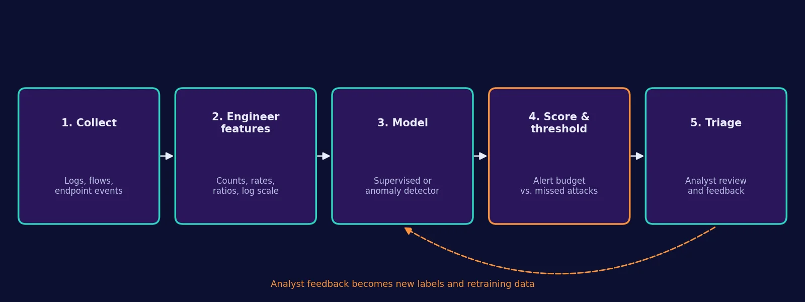
Every ML-based detector follows roughly this flow:

1. Collect: gather logs, network flows, or endpoint events.
2. Engineer features: turn raw events into numbers, such as bytes sent, failed logins per minute, or distinct ports contacted.
3. Model: train a classifier or an anomaly detector.
4. Score and threshold: convert model output into alerts. This is where you decide how many false alarms you can afford.
5. Triage: analysts review alerts, and their verdicts become new labels for retraining.

Most real-world failures happen in steps 1, 2, and 4, not in the choice of algorithm.

Supervised vs Unsupervised: Which Approach Fits?

Approach	Needs labelled attacks?	Good at	Weak at
Supervised classification (e.g. Random Forest)	Yes	Known attack types with many examples	Attacks unlike anything in the training data
Unsupervised / anomaly detection (e.g. Isolation Forest)	No	Unusual behaviour, including novel attacks	Higher false alarms; “unusual” is not always “malicious”
Semi-supervised (train on clean normal data only)	No attacks, but needs clean data	Modelling a stable baseline	Breaks if the “clean” data is contaminated

scikit-learn’s documentation draws a related distinction: outlier detection assumes the training data may contain anomalies, while novelty detection assumes training data is clean and asks whether new observations are unusual (scikit-learn: Novelty and Outlier Detection). In security this matters, because your “normal” logs may already contain an attacker.

How Isolation Forest Finds Anomalies

Isolation Forest, introduced by Liu, Ting, and Zhou, is built on a simple observation: anomalies are few and different, so they are easier to separate from the rest of the data.

The algorithm builds many random trees. Each split picks a random feature and a random threshold. A point in a dense cluster needs many splits to be isolated, while an outlier is usually isolated after only a few. The shorter the average path, the more anomalous the point.

The anomaly score for a point $x$ in a sample of $n$ points is:

$$s(x, n) = 2^{-\frac{E[h(x)]}{c(n)}}$$

• $h(x)$ is the number of splits needed to isolate $x$ in one tree, and $E[h(x)]$ is its average over all trees.
• $c(n)$ is the average path length of an unsuccessful search in a binary search tree, used to normalise scores across sample sizes.
• A score close to 1 suggests an anomaly, and a score well below 0.5 suggests a normal point.

scikit-learn exposes this through IsolationForest, and its contamination parameter controls the share of training points treated as anomalous when setting the decision threshold.

Why Accuracy Is the Wrong Metric: A Worked Example

Suppose a network produces 1,000,000 events per day and 0.01% are malicious, which is 100 attacks. Your detector has 99% recall (it catches 99 of the 100) and a 1% false positive rate. That sounds excellent.

• True positives: 99
• Benign events: 999,900, so false positives are about 1% of that, roughly 9,999
• Precision = 99 / (99 + 9,999) ≈ 0.98%

Fewer than 1 in 100 alerts would be real. Analysts would learn to ignore the system. This is the base rate problem, and it is why security teams care about precision, recall, and the false alarm rate together:

$$\text{Precision} = \frac{TP}{TP + FP}, \qquad \text{Recall} = \frac{TP}{TP + FN}, \qquad F_1 = \frac{2 \cdot \text{Precision} \cdot \text{Recall}}{\text{Precision} + \text{Recall}}$$

Here $TP$ are true positives (real attacks flagged), $FP$ are false positives (benign events flagged), and $FN$ are false negatives (attacks missed).

Hands-On: Supervised vs Anomaly Detection in Python

Now let’s compare both approaches on a small synthetic dataset. The goal is to test one idea: what happens when an attack type was never seen during training?

What the experiment does

• Generates network-flow-style features: duration, bytes sent and received, packets, failed logins, and distinct ports contacted.
• Creates four traffic types: normal, port scan, brute force, and data exfiltration.
• Trains a Random Forest on normal, port scan, and brute force traffic only.
• Trains an Isolation Forest on normal traffic only.
• Tests both on all four types, including exfiltration, which the Random Forest never saw.

Setup

pip install scikit-learn pandas numpy

The output below was produced with Python and these versions: scikit-learn 1.8.0, pandas 3.0.2, NumPy 2.4.4. Other versions may give slightly different numbers.

The code

import numpy as np, pandas as pd
from sklearn.ensemble import IsolationForest, RandomForestClassifier
from sklearn.preprocessing import StandardScaler
from sklearn.metrics import classification_report, precision_score, recall_score, f1_score

rng = np.random.default_rng(42)

def make_normal(n):
    return pd.DataFrame({
        "duration_s":     rng.lognormal(1.5, 0.8, n),
        "bytes_sent":     rng.lognormal(7.0, 1.0, n),
        "bytes_received": rng.lognormal(8.0, 1.1, n),
        "packets":        rng.poisson(40, n) + 1,
        "failed_logins":  rng.poisson(0.05, n),
        "distinct_ports": rng.poisson(1.5, n) + 1,
    }).assign(label="normal")

def make_port_scan(n):
    return pd.DataFrame({
        "duration_s":     rng.lognormal(0.2, 0.5, n),
        "bytes_sent":     rng.lognormal(5.0, 0.5, n),
        "bytes_received": rng.lognormal(4.5, 0.6, n),
        "packets":        rng.poisson(120, n) + 1,
        "failed_logins":  rng.poisson(0.05, n),
        "distinct_ports": rng.poisson(60, n) + 10,
    }).assign(label="port_scan")

def make_brute_force(n):
    return pd.DataFrame({
        "duration_s":     rng.lognormal(2.0, 0.6, n),
        "bytes_sent":     rng.lognormal(6.5, 0.6, n),
        "bytes_received": rng.lognormal(7.0, 0.7, n),
        "packets":        rng.poisson(90, n) + 1,
        "failed_logins":  rng.poisson(12, n) + 3,
        "distinct_ports": rng.poisson(1.2, n) + 1,
    }).assign(label="brute_force")

def make_exfil(n):  # never shown to the supervised model
    return pd.DataFrame({
        "duration_s":     rng.lognormal(2.8, 0.6, n),
        "bytes_sent":     rng.lognormal(10.2, 0.6, n),
        "bytes_received": rng.lognormal(6.5, 0.8, n),
        "packets":        rng.poisson(70, n) + 1,
        "failed_logins":  rng.poisson(0.05, n),
        "distinct_ports": rng.poisson(1.5, n) + 1,
    }).assign(label="data_exfiltration")

train = pd.concat([make_normal(6000), make_port_scan(300), make_brute_force(300)], ignore_index=True)
test  = pd.concat([make_normal(2000), make_port_scan(100), make_brute_force(100), make_exfil(100)], ignore_index=True)
feats = [c for c in train.columns if c != "label"]

def prep(df):
    X = df[feats].copy()
    for c in ["duration_s", "bytes_sent", "bytes_received"]:
        X[c] = np.log1p(X[c])
    return X

scaler = StandardScaler().fit(prep(train[train.label == "normal"]))
X_train, X_test = scaler.transform(prep(train)), scaler.transform(prep(test))
y_train = (train.label != "normal").astype(int)
y_test  = (test.label  != "normal").astype(int)

rf = RandomForestClassifier(n_estimators=200, class_weight="balanced", random_state=42).fit(X_train, y_train)
rf_pred = rf.predict(X_test)

iso = IsolationForest(n_estimators=300, contamination=0.02, random_state=42)
iso.fit(X_train[(train.label == "normal").values])
iso_pred = (iso.predict(X_test) == -1).astype(int)

rows = []
for name, pred in [("Random Forest (supervised)", rf_pred), ("Isolation Forest (normal-only)", iso_pred)]:
    rec = {a: pred[(test.label == a).values].mean() for a in ["port_scan", "brute_force", "data_exfiltration"]}
    rows.append({"model": name,
                 "precision": precision_score(y_test, pred),
                 "recall_overall": recall_score(y_test, pred),
                 "f1": f1_score(y_test, pred),
                 "false_alarm_rate": pred[(test.label == "normal").values].mean(),
                 **{f"recall_{k}": v for k, v in rec.items()}})
res = pd.DataFrame(rows).set_index("model").round(3)
pd.set_option("display.width", 200); pd.set_option("display.max_columns", 20)
print(res.T)
res.to_csv("results.csv")

Results

Running the script above prints (rounded to three decimals):

Metric	Random Forest (supervised)	Isolation Forest (normal-only)
Precision	1.000	0.867
Overall recall	0.740	0.913
F1	0.851	0.890
False alarm rate	0.000	0.021
Recall: port scan	1.000	1.000
Recall: brute force	1.000	1.000
Recall: data exfiltration (unseen)	0.220	0.740

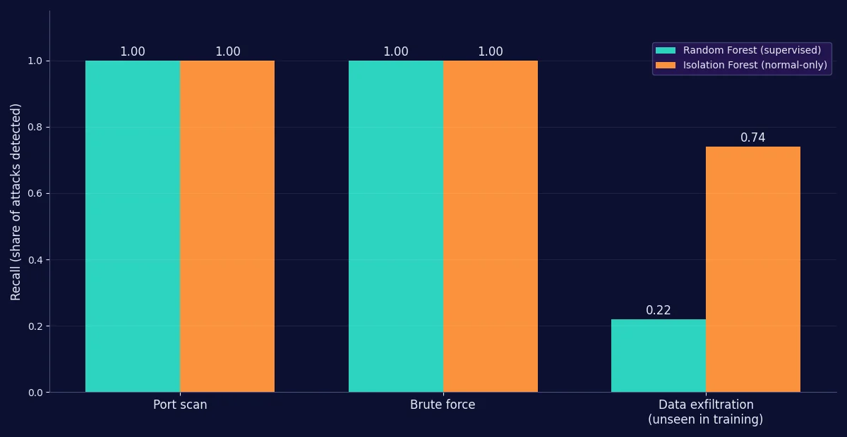
How to read these results

• On known attacks, the supervised model is perfect. It scored zero false alarms and caught every port scan and brute-force event.
• On the unseen attack, it mostly fails. It detected only 22% of exfiltration events, because nothing in its training data resembled them.
• The anomaly detector generalises better but is noisier. It caught 74% of exfiltration and flagged about 2.1% of normal traffic, which is close to the contamination=0.02 setting.

Important limitations of this experiment

This is a teaching demo, not a benchmark.

• The data is synthetic and simple. The distributions were chosen by the author, so the clean separation of port scans and brute force is unrealistically easy.
• The test set is about 13% attacks, far above real-world prevalence. With realistic rates, the Isolation Forest’s 2.1% false alarm rate would produce a precision collapse like the worked example above.
• Results come from one random seed and one split. They show a pattern, not a general ranking of the two algorithms.
• Real traffic drifts over time, and attackers adapt.

To test on realistic data, try a public intrusion-detection dataset such as CIC-IDS2017, and evaluate with a time-based split rather than a random one.

Common Mistakes and Troubleshooting

• Training the anomaly detector on contaminated data. If your “normal” logs include an ongoing intrusion, the model learns it as normal. Clean or review the baseline.
• Setting contamination by guesswork. It directly controls how many events are flagged. Choose it from your alert budget, not from the real attack rate, which you rarely know.
• Random train/test splits on time-ordered data. This leaks future patterns into training. Split by time.
• Skipping scaling or log transforms. Byte counts span orders of magnitude. The script uses log1p and standardisation for that reason.
• Reporting only accuracy. Always report precision, recall, and the false alarm rate, ideally per attack type.
• Using labels from one network on another. Models rarely transfer between environments without retraining.

Where ML Threat Detection Falls Short

• Explainability. Analysts need to know why an event was flagged. Research on user and entity behaviour analytics argues that autoencoders can be more explainable than some other deep models, and explainability is an active research focus (Fuentes, 2025).
• Anomaly is not the same as malicious. A new software rollout or a quarterly backup can look strange and be harmless. Sommer and Paxson made this argument for network intrusion detection in “Outside the Closed World” (IEEE S&P, 2010).
• Adversarial evasion. Attackers can shape their behaviour to resemble normal traffic.
• Data drift. Normal changes, so models need monitoring and periodic retraining.
• Label scarcity. Confirmed attacks are rare and expensive to label.

For a broader view of managing these risks, see the NIST AI Risk Management Framework, and map detections to attacker behaviour using MITRE ATT&CK.

Implementation Checklist

• Define the threat you want to detect and the data that would reveal it.
• Set an alert budget: how many alerts per day can your team review?
• Build a baseline with simple rules or statistics first.
• Engineer features and split data by time.
• Evaluate precision, recall, and false alarm rate per attack type.
• Hold out an attack type to test generalisation, as in the demo above.
• Add explanations (top contributing features) to each alert.
• Monitor drift and plan retraining.
• Capture analyst feedback as labels.

Frequently Asked Questions

Can machine learning detect zero-day attacks?

Sometimes. Anomaly detection can flag behaviour that is unusual even if the specific attack is new, as the demo shows (74% recall on the unseen attack). It cannot guarantee detection, and it will also flag harmless novelty.

Is supervised or unsupervised learning better for cybersecurity?

Neither is better in general. Supervised models are strong on well-labelled, known attack types, and anomaly detectors help with unknown behaviour. Many production systems combine both with rules.

What is the best algorithm for threat detection?

There is no single best algorithm. Isolation Forest is a good starting point for tabular anomaly detection because it is fast and has few parameters, but the right choice depends on your data, labels, and alert budget.

Why do ML security systems create so many false positives?

Because malicious events are extremely rare. Even a small false positive rate, applied to millions of benign events, can outnumber true detections, as the worked example above shows.

Do I need deep learning for threat detection?

Not to get started. Tree-based models and Isolation Forest often work well on structured features. Deep learning, such as autoencoders, becomes more useful with large volumes of raw or sequential data.

Next Steps

Take the script and change one thing at a time: shift the exfiltration distribution closer to normal traffic and watch recall fall, or lower contamination and watch false alarms drop. Then move to a public dataset and a time-based split. The habit to build is the one the experiment shows: always test on an attack your model has not seen.

References

• scikit-learn documentation, Novelty and Outlier Detection.
• Liu, F. T., Ting, K. M., and Zhou, Z.-H. “Isolation Forest.” IEEE International Conference on Data Mining (ICDM), 2008. DOI: 10.1109/ICDM.2008.17.
• Sommer, R. and Paxson, V. “Outside the Closed World: On Using Machine Learning for Network Intrusion Detection.” IEEE Symposium on Security and Privacy, 2010.
• Fuentes, J. “Cybersecurity Threat Detection Based on a UEBA Framework Using Deep Autoencoders.” arXiv:2505.11542.
• NIST, AI Risk Management Framework.
• MITRE, ATT&CK.
• Canadian Institute for Cybersecurity, CIC-IDS2017 dataset.