Linear Algebra for Machine Learning: Vectors, Matrices, and Eigenvalues

If you have ever wondered why machine learning tutorials throw around words like “dot product”, “weight matrix”, or “eigenvalue”, the answer is simple: linear algebra is the language models use to handle data. A table of numbers is a matrix, one row of it is a vector, and most of what a model does to that table is matrix multiplication.

This guide explains linear algebra for machine learning from the ground up. You will learn what vectors and matrices are, how dot products and matrix multiplication work, what eigenvalues and eigenvectors actually mean, and where each idea shows up in real ML code. Every concept comes with a short NumPy example.

What you will learn:

• How vectors represent data points and how the dot product measures similarity
• How matrix multiplication powers linear models and neural network layers
• What eigenvalues and eigenvectors are, geometrically and in code
• How PCA uses eigenvectors of a covariance matrix to reduce dimensions
• Common mistakes that cause shape errors and confusing results

Prerequisites: basic Python and high-school algebra. No prior linear algebra needed.

Setup

You only need NumPy. The PCA comparison near the end also uses scikit-learn, which is optional.

pip install numpy scikit-learn

import numpy as np
np.set_printoptions(precision=4, suppress=True)  # tidier printed output

The examples were run with NumPy 2.4.4 on Python 3.12, and the outputs shown below are the real outputs from that run. They should also work on other recent NumPy versions.

Why Linear Algebra Matters in Machine Learning

Machine learning models need numbers. Images become grids of pixel values, text becomes numeric embeddings, and a customer record becomes a list of features. Linear algebra gives you a compact way to store those numbers and a set of operations to transform them efficiently.

ML task	Linear algebra concept
Represent one data sample	Vector
Represent a dataset	Matrix (rows = samples, columns = features)
Linear regression prediction	Dot product
Neural network dense layer	Matrix multiplication plus a bias
Measuring similarity (search, embeddings)	Dot product, cosine similarity
Dimensionality reduction (PCA)	Eigenvectors and eigenvalues

Vectors: Data Points as Lists of Numbers

A vector is an ordered list of numbers. In ML, a vector usually holds the features of one sample. A house described by [area, bedrooms, age] is a vector with three entries, or a point in 3-dimensional space.

x = np.array([3.0, 4.0])
print(x.shape)            # (2,)
print(np.linalg.norm(x))  # 5.0

(2,)
5.0

The norm (length) of a vector is its distance from the origin. For [3, 4] it is √(3² + 4²) = 5. Norms appear in ML whenever you measure error or regularize weights (L2 regularization penalizes the squared norm of the weights).

Vector addition and scaling

Vectors of the same length add element by element, and multiplying by a number (a scalar) scales every entry.

a = np.array([1, 2, 3])
b = np.array([4, 5, 6])

print(a + b)   # [5 7 9]
print(2 * a)   # [2 4 6]

The dot product

The dot product multiplies matching entries and adds them up:

a · b = a₁b₁ + a₂b₂ + ... + aₙbₙ

print(a @ b)         # 32  (1*4 + 2*5 + 3*6)
print(np.dot(a, b))  # 32

The geometric meaning is more useful than the formula. The dot product equals ‖a‖ ‖b‖ cos(θ), where θ is the angle between the vectors. So it is large and positive when two vectors point in a similar direction, zero when they are perpendicular (orthogonal), and negative when they point in opposite directions.

u = np.array([1, 0])
v = np.array([0, 1])
print(u @ v)  # 0  -> orthogonal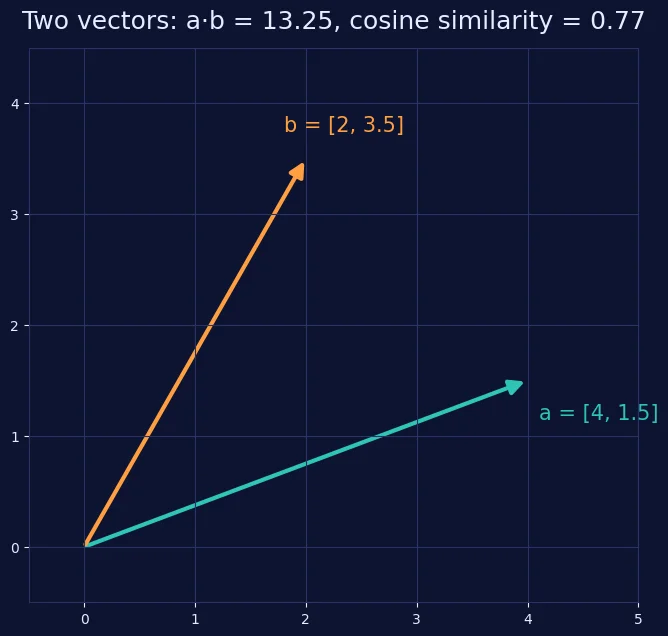

Dividing the dot product by both lengths removes the effect of magnitude and leaves only the angle. This is cosine similarity, widely used to compare text and image embeddings:

cos = (a @ b) / (np.linalg.norm(a) * np.linalg.norm(b))
print(cos)  # 0.9746318461970762

Where it appears in ML: a linear regression prediction is ŷ = w · x + b. Every neuron in a neural network computes the same thing before applying an activation function.

Matrices: Datasets and Transformations

A matrix is a 2D grid of numbers. It plays two roles that are worth keeping separate in your mind:

1. A container for data. A dataset with m samples and n features is an m × n matrix.
2. A transformation. Multiplying a vector by a matrix moves, rotates, stretches, or projects it.

A = np.array([[1, 2],
              [3, 4]])
print(A.T)  # transpose: rows become columns

[[1 3]
 [2 4]]

Matrix Multiplication

Matrix multiplication is the most important operation in deep learning. Entry (i, j) of the result is the dot product of row i of the first matrix with column j of the second.

A = np.array([[1, 2],
              [3, 4]])
B = np.array([[0, 1],
              [1, 0]])

print(A @ B)

[[2 1]
 [4 3]]

Check the top-left entry: row [1, 2] · column [0, 1] = 1·0 + 2·1 = 2. ✓

The shape rule

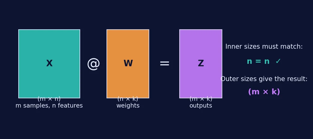
You can multiply an (m × n) matrix by an (n × k) matrix. The two inner sizes must match, and the result is (m × k).

Three facts that trip beginners up

• Order matters. A @ B is generally not equal to B @ A. With the matrices above, B @ A gives [[3, 4], [1, 2]], which swaps the rows of A instead of its columns.
• * is not matrix multiplication. In NumPy, A * B multiplies element by element. Use @ (or np.matmul) for matrix products.
• Shapes must be compatible. Most NumPy errors here are shape mismatches, so check .shape first.

Worked example: a dense layer

A neural network layer (or a multi-output linear model) computes Z = X @ W + b. Here, 2 samples with 3 features each feed a layer with 2 outputs:

X = np.array([[1, 2, 3],
              [4, 5, 6]])            # (2, 3): 2 samples, 3 features
W = np.array([[0.1, 0.2],
              [0.3, 0.4],
              [0.5, 0.6]])           # (3, 2): 3 inputs -> 2 outputs
b = np.array([0.5, -0.5])            # (2,): one bias per output

Z = X @ W + b
print(Z)

[[2.7 2.3]
 [5.4 5.9]]

One matrix multiplication processed every sample at once. This is why GPUs, which are very good at large matrix products, are so central to deep learning. The + b step uses NumPy broadcasting to add the bias vector to each row.

Eigenvalues and Eigenvectors

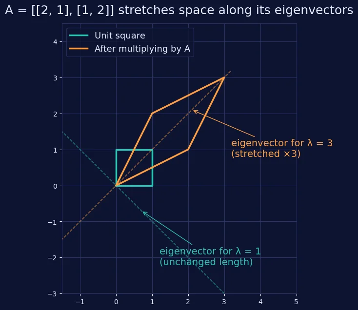
Most vectors change direction when you multiply them by a matrix. Eigenvectors are the special ones that do not. They only get stretched or shrunk (and possibly flipped), and the eigenvalue is the stretch factor.

Formally, for a square matrix A, a non-zero vector v is an eigenvector with eigenvalue λ (lambda) if:

A v = λ v

In words: applying A to v gives the same result as just scaling v by λ.

Finding them with NumPy

S = np.array([[2, 1],
              [1, 2]])

vals, vecs = np.linalg.eig(S)
print(vals)
print(vecs)

[3. 1.]
[[ 0.7071 -0.7071]
 [ 0.7071  0.7071]]

The eigenvalues are 3 and 1. According to the NumPy documentation, the eigenvectors are returned as the columns of vecs, normalized to unit length, so vecs[:, i] pairs with vals[i]. The eigenvalues are not guaranteed to come back in any particular order.

Verify the definition directly:

for i in range(2):
    print(np.allclose(S @ vecs[:, i], vals[i] * vecs[:, i]))

True
True

Reading the result: along [1, 1] the matrix stretches space by a factor of 3, and along [1, -1] it leaves length unchanged (factor 1). That is exactly what the figure above shows.

eig or eigh?

Covariance matrices (and other symmetric matrices) are common in ML, and NumPy has a dedicated function for them, np.linalg.eigh. It is designed for symmetric or Hermitian matrices and returns eigenvalues in ascending order:

vals, vecs = np.linalg.eigh(S)
print(vals)  # [1. 3.]

Use eigh for symmetric matrices. Use eig for general square matrices.

Not every matrix has real eigenvectors

A 90-degree rotation changes every vector’s direction, so no real eigenvector exists. NumPy reports complex eigenvalues instead:

R = np.array([[0, -1],
              [1,  0]])
print(np.linalg.eig(R)[0])  # [0.+1.j 0.-1.j]

If you see complex numbers where you expected real ones, check whether your matrix is symmetric.

Putting It Together: PCA with Eigenvectors

Principal Component Analysis (PCA) reduces the number of features while keeping as much variation as possible. It is a direct application of everything above:

1. Center the data by subtracting each column’s mean.
2. Compute the covariance matrix, a symmetric matrix describing how features vary together.
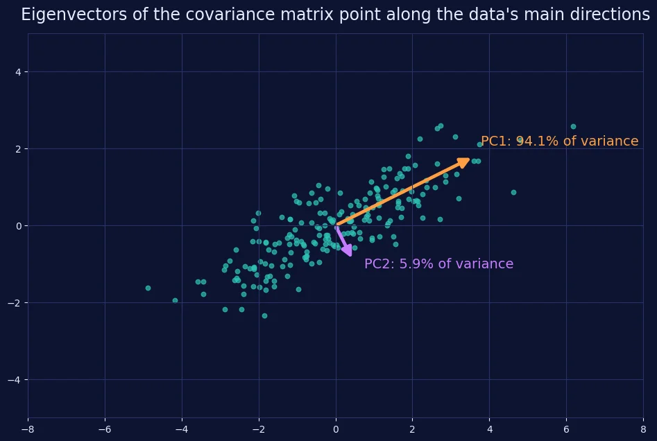
3. Compute its eigenvalues and eigenvectors. Each eigenvector is a direction in feature space, and its eigenvalue is the variance of the data along that direction.
4. Sort by eigenvalue (largest first) and keep the top k eigenvectors.
5. Project the data onto them with a matrix multiplication.

Here is a small, self-contained example using synthetic correlated data:

rng = np.random.default_rng(42)
n = 200
z = rng.normal(size=n)
X = np.column_stack([
    z * 2 + rng.normal(scale=0.5, size=n),
    z * 1 + rng.normal(scale=0.5, size=n),
])

Xc = X - X.mean(axis=0)                   # 1. center
C = np.cov(Xc, rowvar=False)              # 2. covariance matrix (2 x 2)

vals, vecs = np.linalg.eigh(C)            # 3. eigen-decomposition
order = np.argsort(vals)[::-1]            # 4. sort, largest first
vals, vecs = vals[order], vecs[:, order]

print("Eigenvalues:", vals)
print("Variance explained:", vals / vals.sum())

X_1d = Xc @ vecs[:, :1]                   # 5. project onto PC1
print(X_1d.shape)

Eigenvalues: [3.9875 0.2516]
Variance explained: [0.9407 0.0593]
(200, 1)

The first principal component captures about 94% of the variance, so we can compress two correlated features into one while losing little information.

Cross-check with scikit-learn

from sklearn.decomposition import PCA

pca = PCA(n_components=2).fit(X)
print(pca.explained_variance_)   # [3.9875 0.2516]
print(pca.components_)

The explained variances match our eigenvalues. The components may differ by a sign (for example [0.8951, 0.4459] versus [-0.8951, -0.4459]). That is fine: if v is an eigenvector, so is -v. Do not treat the sign as meaningful.

Note: scikit-learn’s PCA is implemented with a singular value decomposition (SVD) of the centered data rather than by explicitly building the covariance matrix. The results agree mathematically, and the covariance-eigenvector route is the clearest way to learn the idea.

Common Mistakes and Troubleshooting

Problem	Cause	Fix
ValueError: shapes (2,3) and (2,3) not aligned	Inner dimensions do not match	Check .shape; transpose one operand if the math calls for it
Result looks wrong but no error	Used * instead of @	Use @ or np.matmul for matrix products
Eigenvectors “do not match” a textbook	Sign flips or different ordering	Verify A @ v == λ * v instead of comparing raw numbers
Eigenvectors look like rows	Misreading the output	NumPy returns eigenvectors as columns (vecs[:, i])
Complex numbers from eig	Matrix is not symmetric (or has rotation)	Use eigh for symmetric matrices; accept complex values otherwise
(n,) vs (n, 1) confusion	1D array is neither a row nor a column	Use .reshape(-1, 1) when you need an explicit column vector
PCA results dominated by one feature	Features on very different scales	Standardize features before PCA

Limitations to Keep in Mind

• Linear algebra describes linear relationships. Neural networks get their expressive power from combining matrix multiplications with non-linear activation functions.
• PCA only finds linear structure and is sensitive to feature scaling.
• Eigendecomposition applies to square matrices. For rectangular matrices, such as raw datasets, the related tool is singular value decomposition (SVD).
• Numerical precision matters. Floating-point arithmetic means results like 1e-16 instead of 0 are normal. Use np.allclose rather than ==.

Quick Reference

Concept	NumPy	ML use
Vector length	np.linalg.norm(v)	Regularization, distances
Dot product	a @ b	Linear models, similarity
Matrix product	A @ B	Neural network layers
Transpose	A.T	Gradients, shape alignment
Eigenvalues/vectors (general)	np.linalg.eig(A)	Stability analysis, spectral methods
Eigenvalues/vectors (symmetric)	np.linalg.eigh(A)	PCA, covariance analysis
Covariance matrix	np.cov(X, rowvar=False)	PCA, statistics

Practice Exercises

1. Compute the cosine similarity between [1, 0, 1] and [1, 1, 0]. What does the result tell you about their directions?
2. Create a random (4, 3) matrix and a (3, 2) matrix. Predict the product’s shape before running @.
3. For M = [[4, 0], [0, 1]], predict the eigenvalues, then confirm with np.linalg.eig.
4. Run the PCA example with scale=2.0 for the noise term. How does the variance explained by PC1 change, and why?

Where to Go Next

Once vectors, matrices, and eigenvalues feel comfortable, the natural next topics are singular value decomposition, gradient descent (which relies on derivatives of matrix expressions), and building a neural network from scratch with NumPy. For a structured course, Mathematics for Machine Learning: Linear Algebra on Coursera covers the same foundations with more proof-based depth.

Frequently Asked Questions

Do I need linear algebra to learn machine learning? You can run models without it, but understanding vectors, matrices, and eigenvalues makes it far easier to debug shape errors, interpret PCA, and follow how neural networks work.

What is the difference between a vector and a matrix? A vector is a one-dimensional list of numbers, and a matrix is a two-dimensional grid. A vector can be viewed as a matrix with one row or one column.

What do eigenvalues tell you in machine learning? Eigenvalues measure how much a transformation stretches space along its eigenvectors. In PCA, the eigenvalues of the covariance matrix give the variance captured by each principal component.

Why does matrix multiplication order matter? Each result entry pairs a row of the first matrix with a column of the second, so swapping the operands changes both the pairing and, often, whether the shapes are even compatible.

References

• NumPy documentation: numpy.linalg.eig: definition of eigenvalues and eigenvectors in NumPy, column convention, and ordering behavior.
• NumPy documentation: numpy.linalg: reference for eigh, norm, and related functions.
• scikit-learn documentation: sklearn.decomposition.PCA: PCA API and implementation notes.
• Strang, G. Linear Algebra and Its Applications: classic textbook reference cited by the NumPy eig documentation.