Backpropagation Explained: How Neural Networks Learn

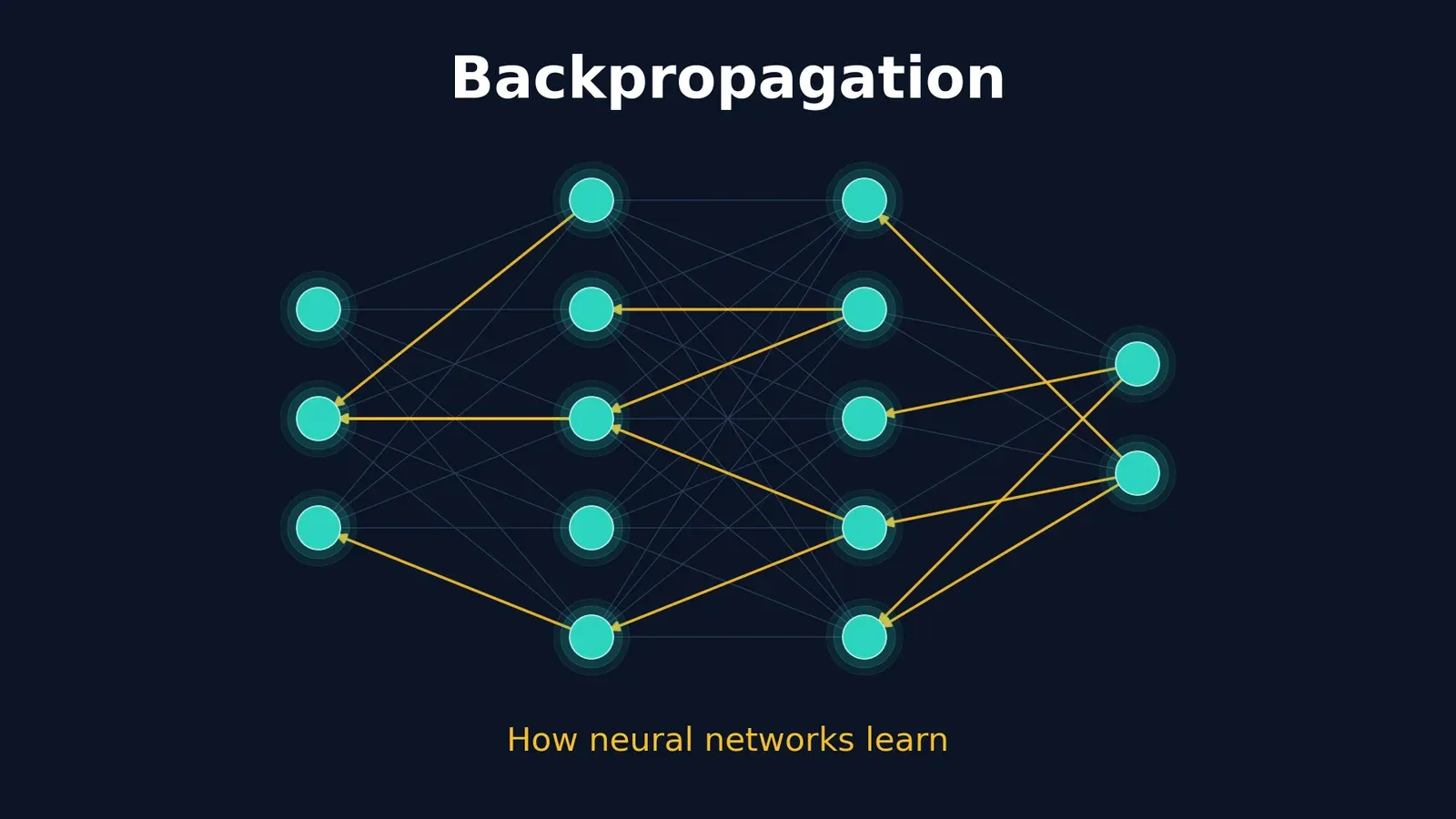
A neural network can have millions or billions of weights, and every one of them has to be nudged in the right direction after each mistake. Backpropagation is the algorithm that tells each weight which direction to move and by how much, using one backward sweep through the network instead of millions of separate experiments.

This article explains backpropagation in layers. You will start with the intuition, then see the exact equations, then follow a complete calculation with real numbers, and finally implement it in NumPy and check it against numerical gradients.

After reading, you will be able to:

• Explain what backpropagation computes and what it does not do.
• Apply the chain rule to a small network by hand.
• Write the four backpropagation equations and say what each one means.
• Implement a working network from scratch and verify its gradients.
• Recognise why gradients vanish, explode, or silently go wrong.

What is backpropagation? (the short answer)

Backpropagation computes the gradient of the loss with respect to every parameter in a neural network. It does this by applying the chain rule of calculus layer by layer, starting at the output and moving backward, reusing intermediate values saved during the forward pass.

It is not a learning algorithm on its own. Backpropagation answers the question “how does the loss change if I change this weight?” A separate step, usually gradient descent or a variant, then uses that answer to update the weights. Keeping these two jobs apart removes a great deal of confusion.

Prerequisites

You need three ideas. If any of them feels shaky, a quick refresher will make the rest of the article much easier.

• Derivatives and the chain rule. If $y = f(g(x))$, then $\frac{dy}{dx} = f'(g(x)) \cdot g'(x)$.
• Partial derivatives and gradients. The gradient of a function is the vector of its partial derivatives. It points in the direction of steepest increase.
• Matrix–vector multiplication. Each layer in this article is a matrix multiplication followed by a non-linear function.

The learning loop at a glance

Training a network repeats four steps:

1. Forward pass. Feed an input through the network and compute a prediction. Save the intermediate values.
2. Loss. Measure how wrong the prediction is with a single number.
3. Backward pass (backpropagation). Compute the gradient of the loss with respect to every weight and bias.
4. Update. Move each parameter a small step against its gradient.

Backpropagation is step 3 only. The rest of this article zooms into it.

Why not just measure each gradient directly?

A natural question is why we need a special algorithm. You could estimate each gradient by nudging one weight slightly and re-measuring the loss. This is called a finite-difference approximation:

$$\frac{\partial L}{\partial w} \approx \frac{L(w + \epsilon) - L(w - \epsilon)}{2\epsilon}$$

The problem is cost. Each estimate needs two extra forward passes, and you need one estimate per parameter. For a model with a million weights, that is two million forward passes for a single update step.

Backpropagation produces all the gradients in one backward pass, whose cost is typically a small constant multiple of the cost of the forward pass. That difference is what makes training large networks feasible. Finite differences are still useful, but as a debugging tool, which we will use later.

The core idea: the chain rule on a computation graph

A neural network is a chain of simple functions. The input goes through layer 1, the result goes through layer 2, and so on until the loss is computed. The loss is therefore a nested function of the weights.

Consider a three-step chain: $w \rightarrow z \rightarrow a \rightarrow L$, where $z = wx$, $a = \sigma(z)$, and $L = \tfrac{1}{2}(a - y)^2$. To find how $L$ responds to $w$, multiply the local sensitivities along the path:

$$\frac{\partial L}{\partial w} = \frac{\partial L}{\partial a} \cdot \frac{\partial a}{\partial z} \cdot \frac{\partial z}{\partial w}$$

Each factor is easy on its own: $\frac{\partial L}{\partial a} = a - y$, $\frac{\partial a}{\partial z} = \sigma'(z)$, and $\frac{\partial z}{\partial w} = x$.

The trick that makes backpropagation efficient is reuse. Many weights share the same downstream path to the loss. Instead of recomputing the downstream part for each weight, backpropagation computes it once and passes it backward. That passed-back quantity is called the error signal, written $\delta$.

Notation

For a network with layers $l = 1, \dots, L$:

Symbol	Meaning
$a^{(0)} = x$	The input vector
$W^{(l)}, b^{(l)}$	Weight matrix and bias vector of layer $l$
$z^{(l)} = W^{(l)} a^{(l-1)} + b^{(l)}$	Pre-activation of layer $l$
$a^{(l)} = \sigma(z^{(l)})$	Activation of layer $l$
$L$	Scalar loss for one example
$\delta^{(l)} = \partial L / \partial z^{(l)}$	Error signal of layer $l$
$\odot$	Element-wise (Hadamard) product

The four backpropagation equations

Define the error signal of a layer as the gradient of the loss with respect to that layer’s pre-activation, $\delta^{(l)} = \partial L / \partial z^{(l)}$. Four equations give everything you need:

$$\delta^{(L)} = \nabla_{a^{(L)}} L \odot \sigma'(z^{(L)}) \tag{1}$$ $$\delta^{(l)} = \left( (W^{(l+1)})^{\top} \delta^{(l+1)} \right) \odot \sigma'(z^{(l)}) \tag{2}$$ $$\frac{\partial L}{\partial W^{(l)}} = \delta^{(l)} \, (a^{(l-1)})^{\top} \tag{3}$$ $$\frac{\partial L}{\partial b^{(l)}} = \delta^{(l)} \tag{4}$$

What each one says in plain language:

• Equation 1 starts the process at the output layer: how much does the loss care about the output, scaled by how sensitive the activation is.
• Equation 2 is the “propagation” step. The error signal of layer $l$ is the error signal of layer $l+1$ sent back through the transpose of the weights, then scaled by the local activation slope.
• Equation 3 says a weight’s gradient is the error signal arriving at its output neuron times the activation arriving at its input. A weight connecting a silent neuron (activation near 0) to anything gets almost no gradient.
• Equation 4 is the same for biases, which have an implicit input of 1.

Where equation 2 comes from

Since $z^{(l+1)} = W^{(l+1)} \sigma(z^{(l)}) + b^{(l+1)}$, each $z_j^{(l)}$ influences the loss only through the entries of $z^{(l+1)}$. The chain rule sums over all of those paths:

$$\delta_j^{(l)} = \sum_k \frac{\partial L}{\partial z_k^{(l+1)}} \frac{\partial z_k^{(l+1)}}{\partial z_j^{(l)}} = \sum_k \delta_k^{(l+1)} \, W_{kj}^{(l+1)} \, \sigma'(z_j^{(l)})$$

Written in matrix form, the sum over $k$ becomes multiplication by $(W^{(l+1)})^{\top}$, which gives equation 2. The transpose is not a trick: it is exactly what “send the signal back along the same connections” means.

A complete worked example with real numbers

Let’s apply the equations to the smallest network that still has a hidden layer: 2 inputs, 2 hidden neurons with sigmoid activation, and 1 sigmoid output neuron. We use the loss $L = \tfrac{1}{2}(a^{(2)} - y)^2$.

Setup

• Input $x = (0.5, -1.0)$ and target $y = 1$.
• $W^{(1)} = \begin{pmatrix} 0.1 & 0.4 \\ -0.2 & 0.3 \end{pmatrix}$, $b^{(1)} = (0, 0.1)$.
• $W^{(2)} = (0.5, -0.6)$, $b^{(2)} = 0.2$.

Forward pass

Hidden layer: $z^{(1)} = W^{(1)}x + b^{(1)} = (0.05 - 0.40,\; -0.10 - 0.30 + 0.1) = (-0.35, -0.30)$. Applying the sigmoid gives $a^{(1)} \approx (0.4134, 0.4256)$.

Output layer: $z^{(2)} = 0.5(0.4134) - 0.6(0.4256) + 0.2 \approx 0.1514$, so $a^{(2)} = \sigma(0.1514) \approx 0.5378$.

Loss: $L = \tfrac{1}{2}(0.5378 - 1)^2 \approx 0.1068$.

Backward pass

Use the sigmoid derivative $\sigma'(z) = \sigma(z)\,(1 - \sigma(z))$, which lets us reuse the saved activations.

Step	Computation	Result
Output error signal (eq. 1)	$\delta^{(2)} = (a^{(2)} - y)\, a^{(2)}(1 - a^{(2)})$	$-0.4622 \times 0.2486 \approx -0.1149$
Output weight gradient (eq. 3)	$\delta^{(2)}\, a^{(1)}$	$(-0.0475,\; -0.0489)$
Output bias gradient (eq. 4)	$\delta^{(2)}$	$-0.1149$
Signal sent back (eq. 2, first part)	$(W^{(2)})^{\top}\delta^{(2)}$	$(-0.0574,\; 0.0689)$
Hidden error signal (eq. 2)	multiply by $a^{(1)}(1 - a^{(1)}) \approx (0.2425, 0.2445)$	$\delta^{(1)} \approx (-0.0139,\; 0.0169)$
Hidden weight gradient (eq. 3)	$\delta^{(1)} x^{\top}$	$\begin{pmatrix} -0.0070 & 0.0139 \\ 0.0084 & -0.0169 \end{pmatrix}$
Hidden bias gradient (eq. 4)	$\delta^{(1)}$	$(-0.0139,\; 0.0169)$

Notice two things. The output gradients are negative, which means increasing those weights would decrease the loss, so gradient descent will increase them. And the hidden error signals are much smaller than the output one (about 0.014 and 0.017 versus 0.115), because the error had to pass through the weights and through a sigmoid slope of at most 0.25. We will return to that shrinkage when we discuss vanishing gradients.

One update step

With a learning rate of 0.5, we update each parameter by subtracting $0.5 \times$ its gradient. Re-running the forward pass with the new weights lowers the loss from about 0.1068 to 0.0976.

Verify it with code: gradient checking

Every number above was computed by the script below, and it also compares each analytic gradient with a finite-difference estimate. This check is the single most useful habit when you implement backpropagation yourself.

import numpy as np

def sigmoid(z):
    return 1.0 / (1.0 + np.exp(-z))

x = np.array([0.5, -1.0])
y = 1.0
W1 = np.array([[0.1, 0.4], [-0.2, 0.3]])
b1 = np.array([0.0, 0.1])
W2 = np.array([[0.5, -0.6]])
b2 = np.array([0.2])

def forward(W1, b1, W2, b2):
    z1 = W1 @ x + b1
    a1 = sigmoid(z1)
    z2 = W2 @ a1 + b2
    a2 = sigmoid(z2)
    return z1, a1, z2, a2

# Forward pass and loss
z1, a1, z2, a2 = forward(W1, b1, W2, b2)
loss = (0.5 * (a2 - y) ** 2).item()
print(f"loss = {loss:.4f}")

# Backward pass: equations (1)-(4)
delta2 = (a2 - y) * a2 * (1 - a2)          # eq. 1
dW2 = np.outer(delta2, a1)                  # eq. 3
db2 = delta2                                # eq. 4
delta1 = (W2.T @ delta2) * a1 * (1 - a1)    # eq. 2
dW1 = np.outer(delta1, x)                   # eq. 3
db1 = delta1                                # eq. 4

# Numerical gradient check (central differences)
def numerical_grad(param, eps=1e-6):
    grad = np.zeros_like(param)
    it = np.nditer(param, flags=["multi_index"])
    for _ in it:
        i = it.multi_index
        old = param[i]
        param[i] = old + eps
        plus = (0.5 * (forward(W1, b1, W2, b2)[3] - y) ** 2).item()
        param[i] = old - eps
        minus = (0.5 * (forward(W1, b1, W2, b2)[3] - y) ** 2).item()
        param[i] = old
        grad[i] = (plus - minus) / (2 * eps)
    return grad

for name, param, analytic in [("W1", W1, dW1), ("b1", b1, db1),
                              ("W2", W2, dW2), ("b2", b2, db2)]:
    diff = np.max(np.abs(numerical_grad(param) - analytic))
    print(f"{name}: max |numerical - analytic| = {diff:.2e}")

Expected output (from an actual run with NumPy 2.4.4 on Python 3.12): the loss is about 0.1068 and the maximum difference for every parameter group is on the order of $10^{-11}$, which is consistent with floating-point error. If your own implementation shows differences near $10^{-3}$ or larger, there is almost certainly a bug in the backward pass.

Build a trainable network from scratch (XOR)

XOR is a classic test because a network without a hidden layer cannot solve it, so success proves that backpropagation is training the hidden units. The code below uses the vectorised form of the same equations, a binary cross-entropy loss, and full-batch gradient descent.

For a sigmoid output with binary cross-entropy loss, the sigmoid slope cancels and equation 1 simplifies to $\delta^{(L)} = a^{(L)} - y$. This is one reason that pairing is so popular.

import numpy as np

rng = np.random.default_rng(42)

def sigmoid(z):
    return 1.0 / (1.0 + np.exp(-z))

# XOR dataset: one example per row
X = np.array([[0, 0], [0, 1], [1, 0], [1, 1]], dtype=float)
y = np.array([[0], [1], [1], [0]], dtype=float)

n_in, n_hidden, n_out = 2, 4, 1
W1 = rng.normal(0, 1.0, size=(n_in, n_hidden))
b1 = np.zeros((1, n_hidden))
W2 = rng.normal(0, 1.0, size=(n_hidden, n_out))
b2 = np.zeros((1, n_out))

lr = 1.0
for epoch in range(5001):
    # forward
    z1 = X @ W1 + b1
    a1 = sigmoid(z1)
    z2 = a1 @ W2 + b2
    a2 = sigmoid(z2)

    eps = 1e-12
    loss = -np.mean(y * np.log(a2 + eps) + (1 - y) * np.log(1 - a2 + eps))

    # backward (sigmoid + binary cross-entropy -> dz2 = a2 - y, averaged over batch)
    m = X.shape[0]
    dz2 = (a2 - y) / m
    dW2 = a1.T @ dz2
    db2 = dz2.sum(axis=0, keepdims=True)
    da1 = dz2 @ W2.T
    dz1 = da1 * a1 * (1 - a1)
    dW1 = X.T @ dz1
    db1 = dz1.sum(axis=0, keepdims=True)

    # update
    W1 -= lr * dW1; b1 -= lr * db1
    W2 -= lr * dW2; b2 -= lr * db2

    if epoch in (0, 500, 1000, 2000, 5000):
        print(f"epoch {epoch:5d}  loss {loss:.4f}")

print("predictions:", a2.round(3).ravel())
print("rounded:", (a2 > 0.5).astype(int).ravel(), "targets:", y.astype(int).ravel())

Output from an actual run (seed 42):

epoch     0  loss 0.7568
epoch   500  loss 0.0646
epoch  1000  loss 0.0129
epoch  2000  loss 0.0039
epoch  5000  loss 0.0011
predictions: [0.001 0.999 0.999 0.002]
rounded: [0 1 1 0] targets: [0 1 1 0]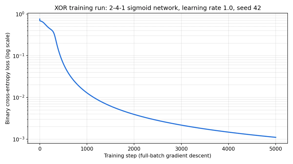

Your exact numbers will differ with another random seed or initialisation, but the downward trend should look similar. Notice the line-by-line correspondence: dz2 is equation 1, da1 = dz2 @ W2.T followed by the multiplication with a1 * (1 - a1) is equation 2, and X.T @ dz1 and a1.T @ dz2 are equation 3. Here the input is stored as rows, so the matrices appear transposed relative to the column-vector equations above.

Backpropagation in a framework: PyTorch autograd

In practice you almost never write the backward pass by hand. Frameworks such as PyTorch record the operations performed during the forward pass as a graph, then walk that graph backward to apply the chain rule automatically. This is called reverse-mode automatic differentiation, and it is the general form of backpropagation.

The snippet below reproduces the worked example, so the gradients it prints should match the table above.

Status: This snippet was reviewed against the PyTorch autograd documentation but not executed while preparing this article. Run it yourself to confirm the output.

import torch

x = torch.tensor([0.5, -1.0])
y = torch.tensor(1.0)

W1 = torch.tensor([[0.1, 0.4], [-0.2, 0.3]], requires_grad=True)
b1 = torch.tensor([0.0, 0.1], requires_grad=True)
W2 = torch.tensor([0.5, -0.6], requires_grad=True)
b2 = torch.tensor(0.2, requires_grad=True)

a1 = torch.sigmoid(W1 @ x + b1)
a2 = torch.sigmoid(W2 @ a1 + b2)
loss = 0.5 * (a2 - y) ** 2

loss.backward()          # runs backpropagation through the recorded graph

print(W1.grad)           # expected to match dW1 from the table
print(W2.grad)           # expected to match dW2 from the table

According to the PyTorch documentation, only leaf tensors with requires_grad=True have their gradients accumulated into the .grad field during the backward pass. The word accumulated matters: calling backward() repeatedly adds to existing gradients, which is why training loops reset them (for example with optimizer.zero_grad()) before each step.

Backpropagation, gradient descent, and optimizers: who does what?

These terms are often used as if they were interchangeable. They are not.

Concept	Question it answers	Example
Backpropagation	What is the gradient of the loss with respect to each parameter?	Equations 1–4
Gradient descent	Given gradients, how should the parameters move?	$w \leftarrow w - \eta \, \partial L / \partial w$
Optimizer	How should the update use gradient history, such as momentum or adaptive step sizes?	SGD with momentum, Adam
Loss function	How is “wrong” measured?	Cross-entropy, mean squared error

You can swap the optimizer without touching backpropagation, and you can compute gradients with backpropagation and never use them for training at all, for example to analyse which input pixels most affect a prediction.

Common problems and how to recognise them

Vanishing gradients

Equation 2 multiplies the error signal by $\sigma'(z)$ at every layer. The sigmoid’s derivative never exceeds 0.25, so the activation-slope factors alone shrink the signal by at least $0.25^{10} \approx 10^{-6}$ across ten sigmoid layers, before the weights are even considered. Early layers then learn extremely slowly. Common remedies include ReLU-family activations, careful weight initialisation, residual connections, and normalisation layers.

Exploding gradients

If the weight matrices have large norms, repeated multiplication can instead make the signal grow without bound. Symptoms are a loss that suddenly becomes NaN or infinity. Gradient clipping and sensible initialisation are standard defences.

Dead ReLUs

For a ReLU activation, $\sigma'(z) = 0$ whenever $z < 0$. A neuron that always receives negative pre-activations passes zero gradient backward and stops learning.

Implementation bugs

• Shape mismatches. Printing the shape of every gradient and checking that it equals the shape of its parameter catches many mistakes.
• Forgetting to reset gradients in frameworks that accumulate them.
• In-place operations. The PyTorch documentation explains that in-place operations can overwrite values needed for gradient computation, and discourages them in most cases.
• Wrong loss and activation pairing, such as applying a sigmoid twice before a loss that already expects raw scores.

When in doubt, run a gradient check like the one earlier in this article on a tiny version of your model.

Common misconceptions

• “Backpropagation sends errors backward as if neurons learn from each other.” It is a bookkeeping method for computing derivatives. There is no claim that biological brains work this way.
• “Backpropagation finds the best weights.” It computes a local slope. Whether training reaches a good solution depends on the loss landscape, the optimizer, and the data.
• “A low training loss means the model works.” Training loss measures fit to the training data. Generalisation must be checked on held-out data.

Practice exercises

1. Compute $\sigma'(0)$. What is the largest value the sigmoid’s derivative can take?
2. ReLU gradient. For a ReLU hidden neuron with $z = -2$, what is its contribution to $\delta^{(l)}$?
3. Cross-entropy shortcut. For a single sigmoid output $a$ with loss $L = -[y\ln a + (1-y)\ln(1-a)]$, show that $\delta^{(L)} = a - y$.

Solutions

1. $\sigma(0) = 0.5$, so $\sigma'(0) = 0.5 \times 0.5 = 0.25$. This is the maximum, because $\sigma(z)(1-\sigma(z))$ is largest when $\sigma(z) = 0.5$.
2. $\text{ReLU}'(z) = 0$ for $z < 0$, so the neuron’s error signal is exactly 0 and its incoming weights receive no gradient for this example.
3. $\frac{\partial L}{\partial a} = -\frac{y}{a} + \frac{1-y}{1-a}$. Multiply by $\sigma'(z) = a(1-a)$ to get $-y(1-a) + (1-y)a = a - y$.

Conclusion

Backpropagation is the chain rule applied efficiently. It saves the values computed in the forward pass, then sweeps backward once, passing an error signal $\delta$ from layer to layer and turning it into a gradient for every weight and bias. A separate optimizer then uses those gradients to update the model.

If you remember only one thing, remember the split of responsibilities: backpropagation computes gradients, and the optimizer decides what to do with them. Once that is clear, vanishing gradients, exploding gradients, and debugging become much easier to reason about.

Suggested next steps:

• Extend the XOR network to a second hidden layer, then use the gradient-check function to verify your new backward pass.
• Replace sigmoid with ReLU and compare how the loss curve and the hidden-layer gradients change.
• Study how backpropagation extends to sequences (backpropagation through time) and to convolutional layers.

Frequently asked questions

Who invented backpropagation?

The 1986 Nature paper by Rumelhart, Hinton, and Williams popularised backpropagation for training multi-layer networks and showed that hidden units learn useful internal representations. The underlying mathematics of reverse-mode differentiation had been developed independently by other researchers earlier, so credit is shared across several contributions.

Is backpropagation the same as gradient descent?

No. Backpropagation computes gradients. Gradient descent uses them to update parameters.

Why is it called “backward” propagation?

The error signal is computed starting at the output layer and moves toward the input layer, in the opposite direction from the forward pass that produces predictions.

Do I need to implement backpropagation by hand?

Not for production work, since frameworks like PyTorch compute gradients automatically. Implementing it once by hand is still valuable because it makes shape errors, gradient flow problems, and loss function choices far easier to understand.

Why does backpropagation need the forward pass values?

Equations 1–3 use the saved activations and pre-activations, for example $\sigma'(z)$ and $a^{(l-1)}$. Frameworks store these during the forward pass, which is part of why training uses more memory than inference.

Does backpropagation work with any activation function?

It needs a derivative (or a defined substitute) almost everywhere. ReLU is not differentiable at exactly zero, so frameworks define a convention there. The PyTorch documentation describes rules for choosing gradients of non-differentiable functions.

What is the difference between backpropagation and backpropagation through time?

Backpropagation through time applies the same idea to recurrent networks by unrolling the network across time steps and backpropagating through the unrolled graph.

References and further reading

• Rumelhart, D. E., Hinton, G. E., & Williams, R. J. (1986). Learning representations by back-propagating errors. Nature, 323(6088), 533–536.
• PyTorch documentation: Autograd mechanics.
• Grant Sanderson (3Blue1Brown): What is backpropagation really doing? A visual walkthrough of the same algorithm.

Code in this article was executed with Python 3.12 and NumPy 2.4.4 except where a snippet is explicitly marked as not executed.