CNN Explained with Python: Build an Image Classifier

A convolutional neural network (CNN) is a neural network that processes images by sliding small learned filters across them, instead of connecting every pixel to every neuron. That one design choice makes image models far more efficient and far better at finding patterns such as edges, textures, and shapes wherever they appear.

In this tutorial you will do three things. First, you will compute a convolution and a pooling step by hand and in NumPy, so the operations stop being mysterious. Second, you will see how those pieces stack into a network and how to predict every layer’s shape and parameter count before running anything. Third, you will build, train, and evaluate a CNN image classifier on Fashion-MNIST in PyTorch, with an equivalent Keras version for TensorFlow users.

You will need: basic Python and NumPy, and a rough idea of what a neural network layer and a loss function are. You do not need prior experience with PyTorch or TensorFlow.

What is a CNN? (the short answer)

A CNN is a stack of layers where the early layers are convolutions and pooling operations that extract spatial features from an image, and the final layers are ordinary fully connected layers that turn those features into class scores.

• A convolutional layer applies a small grid of learned weights (a kernel or filter) at every position of the image and records how strongly the pattern matches. The output is a feature map.
• A pooling layer shrinks each feature map by summarising small neighbourhoods, which reduces computation and makes the representation less sensitive to tiny shifts.
• A fully connected layer at the end combines the extracted features and outputs one score per class.

CNNs were popularised for image recognition by LeCun and colleagues, whose 1998 paper describes convolutional networks trained with backpropagation for handwritten character recognition (Gradient-Based Learning Applied to Document Recognition, Proceedings of the IEEE).

Why not just use a regular neural network on pixels?

You can flatten a 28×28 image into 784 numbers and feed it to a fully connected network. It works on small problems, but it ignores something important: nearby pixels are related, and the same pattern can appear anywhere.

A convolutional layer builds in two assumptions that suit images:

• Local connectivity. Each output value depends only on a small patch of the input, such as 3×3 pixels, not the whole image.
• Weight sharing. The same kernel is reused at every position. A filter that detects a vertical edge in the top-left corner also detects it in the bottom-right.

The result is that a convolutional layer needs very few parameters. In the model we build later, both convolutional layers together have only 4,800 parameters. We will compute that exactly in a moment.

Convolution, step by step

The operation

Take a 2D input $x$ and a small kernel $K$. At each position $(i, j)$, multiply the kernel with the patch of the input beneath it, add up the products, and add a bias $b$:

$$y_{i,j} = b + \sum_{u=0}^{k-1} \sum_{v=0}^{k-1} K_{u,v} \; x_{i+u,\; j+v}$$

Here $k$ is the kernel size. Sliding the kernel over every valid position produces the feature map $y$.

A terminology note. Mathematically, this formula is cross-correlation, not convolution, because the kernel is not flipped. Deep learning libraries use it anyway. The PyTorch documentation for Conv2d describes the operation as a 2D cross-correlation. Since the kernel is learned, the distinction does not matter in practice: the network simply learns whichever orientation it needs.

A worked example you can verify

Consider a 6×6 image whose left half is dark (0) and right half is bright (1), and a 3×3 vertical-edge kernel with columns $(-1, 0, 1)$:

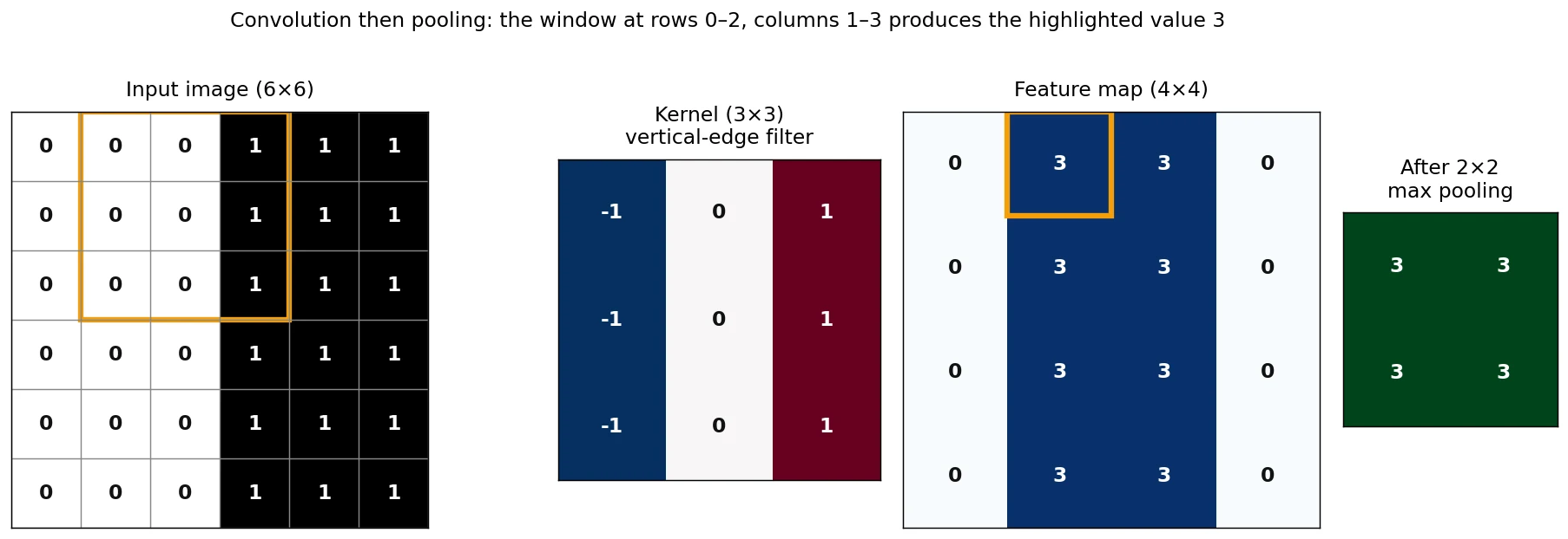
The highlighted window covers rows 0–2 and columns 1–3. In each row it contains the values $(0, 0, 1)$. Multiplying by the kernel row $(-1, 0, 1)$ gives $0 + 0 + 1 = 1$ per row, and three rows add up to 3. At the far left, the window sees only zeros and the output is 0. At the far right, it sees only ones, giving $-1 + 0 + 1 = 0$ per row. The filter responds only where the brightness changes, which is exactly what an edge detector should do.

Here is the same calculation in NumPy:

import numpy as np
from scipy.signal import correlate2d

def conv2d_valid(image, kernel):
    kh, kw = kernel.shape
    out_h = image.shape[0] - kh + 1
    out_w = image.shape[1] - kw + 1
    out = np.zeros((out_h, out_w))
    for i in range(out_h):
        for j in range(out_w):
            patch = image[i:i + kh, j:j + kw]
            out[i, j] = np.sum(patch * kernel)
    return out

image = np.zeros((6, 6))
image[:, 3:] = 1.0                      # dark left half, bright right half
kernel = np.array([[-1, 0, 1],
                   [-1, 0, 1],
                   [-1, 0, 1]], dtype=float)

fmap = conv2d_valid(image, kernel)
print(fmap)
print("matches SciPy:", np.allclose(fmap, correlate2d(image, kernel, mode="valid")))

Output from an actual run (NumPy and SciPy):

[[0. 3. 3. 0.]
 [0. 3. 3. 0.]
 [0. 3. 3. 0.]
 [0. 3. 3. 0.]]
matches SciPy: True

Notice that the 6×6 input produced a 4×4 output. Without padding, a $k \times k$ kernel loses $k - 1$ pixels along each dimension.

Stride, padding, and output size

Two settings control the output size. Stride is how many pixels the kernel moves each step. Padding adds a border of zeros around the input. The PyTorch documentation gives the output height as:

$$H_{out} = \left\lfloor \frac{H_{in} + 2p - d\,(k - 1) - 1}{s} + 1 \right\rfloor$$

where $p$ is padding, $s$ is stride, $k$ is kernel size, and $d$ is dilation (usually 1). With $k = 3$, $s = 1$, and $p = 1$, the output has the same height and width as the input. This is why the model below uses padding=1 with 3×3 kernels.

Channels, filters, and parameter counts

Real images have channels (1 for grayscale, 3 for RGB), and each layer learns many filters, not one. A convolutional layer with in_channels $= C_{in}$, out_channels $= C_{out}$, and kernel size $k$ has weights of shape $(C_{out}, C_{in}, k, k)$ and $C_{out}$ biases. So:

$$\text{parameters} = C_{out} \cdot C_{in} \cdot k^2 + C_{out}$$

For a layer with 1 input channel, 16 filters, and a 3×3 kernel, that is $16 \cdot 1 \cdot 9 + 16 = 160$ parameters, no matter how large the image is. That independence from image size is the payoff of weight sharing.

The activation function

After each convolution, a non-linear activation is applied, usually ReLU, defined as $\max(0, x)$. Without it, stacked convolutions would collapse into one linear operation. In our edge example, ReLU would leave the feature map unchanged because every value is already non-negative. If you flipped the image so the bright half were on the left, the same kernel would produce $-3$ values, and ReLU would set them to zero. The filter then reports only the “dark-to-bright” edge direction, and the network learns other filters for other directions.

Pooling: shrinking while keeping the signal

Max pooling with a 2×2 window and stride 2 splits the feature map into non-overlapping 2×2 blocks and keeps the largest value in each. A 4×4 map becomes 2×2, cutting the number of values by 75%.

def maxpool2d(x, size=2):
    h, w = x.shape
    out = np.zeros((h // size, w // size))
    for i in range(0, h - h % size, size):
        for j in range(0, w - w % size, size):
            out[i // size, j // size] = x[i:i + size, j:j + size].max()
    return out

print(maxpool2d(fmap))

[[3. 3.]
 [3. 3.]]

Pooling provides some tolerance to small shifts, but only partially. The next snippet moves a feature by one pixel, once within a pooling block and once across a block boundary:

a = np.zeros((4, 4)); a[0, 0] = 5.0
b = np.zeros((4, 4)); b[1, 1] = 5.0      # moved, but still inside the same 2x2 block
print(np.array_equal(maxpool2d(a), maxpool2d(b)))      # True

c = np.zeros((4, 4)); c[1, 1] = 5.0
d = np.zeros((4, 4)); d[1, 2] = 5.0      # moved across a block boundary
print(np.array_equal(maxpool2d(c), maxpool2d(d)))      # False

Both comparisons printed the results shown in the comments when run. This is why it is more accurate to say that CNNs gain approximate, local shift tolerance than to claim they are fully translation invariant. Convolution itself is equivariant to shifts (shift the input and the feature map shifts with it, ignoring borders); pooling and the deeper layers add partial invariance.

How layers stack into a hierarchy

Early filters see only small patches, so they learn simple patterns such as edges. Later layers receive feature maps and combine them, so each output value depends on a larger region of the original image. This region is called the receptive field.

For the network we are about to build (3×3 convolution, 2×2 pool, 3×3 convolution, 2×2 pool), the receptive field grows as follows. These values were computed with a short script using the standard recurrence $\text{rf} \leftarrow \text{rf} + (k-1)\cdot\text{jump}$, where jump is the product of earlier strides:

After layer	Receptive field (pixels)
conv1 (3×3)	3×3
pool1 (2×2, stride 2)	4×4
conv2 (3×3)	8×8
pool2 (2×2, stride 2)	10×10

So by the second pooling layer, each feature “sees” a 10×10 patch of a 28×28 image. The deeper layers can respond to parts of objects (a sleeve, a heel) instead of single edges.

Project: build an image classifier with PyTorch

The dataset

We use Fashion-MNIST, a dataset of 28×28 grayscale images of 70,000 fashion products in 10 categories, with 60,000 training images and 10,000 test images (Xiao, Rasul & Vollgraf, 2017). It keeps the format of the classic MNIST digits dataset but is a harder task, and it is small enough to train on modest hardware.

The ten classes are: T-shirt/top, Trouser, Pullover, Dress, Coat, Sandal, Shirt, Sneaker, Bag, and Ankle boot.

Code status. The NumPy snippets above were executed. The PyTorch and Keras code below was reviewed against the official documentation but not executed while this article was prepared, because those libraries and dataset downloads were unavailable in the authoring environment. The layer shapes and parameter counts below were computed by a separate script. Run the code yourself, and treat any accuracy you obtain as your own measurement; this article does not report accuracy numbers.

Install and load the data

pip install torch torchvision

import copy
import torch
from torch import nn
from torch.utils.data import DataLoader, random_split
from torchvision import datasets, transforms

torch.manual_seed(42)
device = "cuda" if torch.cuda.is_available() else "cpu"

transform = transforms.Compose([
    transforms.ToTensor(),                  # uint8 [0, 255] -> float [0, 1], shape (1, 28, 28)
    transforms.Normalize((0.5,), (0.5,)),   # rescale to [-1, 1]
])

full_train = datasets.FashionMNIST("data", train=True, download=True, transform=transform)
test_set = datasets.FashionMNIST("data", train=False, download=True, transform=transform)
class_names = full_train.classes

# Hold out 6,000 training images for validation. The test set stays untouched until the end.
train_set, val_set = random_split(
    full_train, [54_000, 6_000], generator=torch.Generator().manual_seed(42)
)

train_loader = DataLoader(train_set, batch_size=128, shuffle=True)
val_loader = DataLoader(val_set, batch_size=512)
test_loader = DataLoader(test_set, batch_size=512)

Three sets matter here. The training set updates the weights. The validation set guides decisions such as which epoch to keep. The test set is used once, at the end, so that the final number is an honest estimate of performance on unseen data.

Define the model

class SmallCNN(nn.Module):
    def __init__(self, num_classes=10):
        super().__init__()
        self.features = nn.Sequential(
            nn.Conv2d(1, 16, kernel_size=3, padding=1),   # 1x28x28  -> 16x28x28
            nn.ReLU(),
            nn.MaxPool2d(2),                              # 16x28x28 -> 16x14x14
            nn.Conv2d(16, 32, kernel_size=3, padding=1),  # 16x14x14 -> 32x14x14
            nn.ReLU(),
            nn.MaxPool2d(2),                              # 32x14x14 -> 32x7x7
        )
        self.classifier = nn.Sequential(
            nn.Flatten(),                                 # 32*7*7 = 1568 values
            nn.Linear(32 * 7 * 7, 128),
            nn.ReLU(),
            nn.Dropout(0.3),
            nn.Linear(128, num_classes),                  # raw scores (logits)
        )

    def forward(self, x):
        return self.classifier(self.features(x))

model = SmallCNN().to(device)
print(sum(p.numel() for p in model.parameters()))

The model outputs raw scores called logits, not probabilities. PyTorch’s nn.CrossEntropyLoss expects logits and applies the softmax internally, so you should not add a softmax layer before it.

Shapes and parameters (calculated by script from the formulas above):

Layer	Output shape	Parameters
Input	1×28×28	0
Conv2d(1, 16, 3, padding=1)	16×28×28	160
MaxPool2d(2)	16×14×14	0
Conv2d(16, 32, 3, padding=1)	32×14×14	4,640
MaxPool2d(2)	32×7×7	0
Linear(1568, 128)	128	200,832
Linear(128, 10)	10	1,290
Total		206,922

The print in the code should therefore show 206922. If it does not, one of your layer sizes differs from the table.

Look at where the parameters are. The two convolutional layers hold only 4,800 of the 206,922. The first fully connected layer holds almost all the rest. For comparison, a plain 784→128→10 network would have 101,770 parameters, fewer than this CNN. The advantage of the CNN here is not a smaller parameter count. It is that the weights are arranged to exploit image structure, and that its convolutional part is independent of image size.

Train the model

criterion = nn.CrossEntropyLoss()
optimizer = torch.optim.Adam(model.parameters(), lr=1e-3)

def evaluate(loader):
    model.eval()                          # turns off dropout
    total_loss, correct, n = 0.0, 0, 0
    with torch.no_grad():                 # no gradients needed for evaluation
        for x, y in loader:
            x, y = x.to(device), y.to(device)
            logits = model(x)
            total_loss += criterion(logits, y).item() * y.size(0)
            correct += (logits.argmax(dim=1) == y).sum().item()
            n += y.size(0)
    return total_loss / n, correct / n

EPOCHS = 8
best_val_acc, best_state = 0.0, None

for epoch in range(1, EPOCHS + 1):
    model.train()                         # turns dropout on
    running_loss, seen = 0.0, 0
    for x, y in train_loader:
        x, y = x.to(device), y.to(device)
        optimizer.zero_grad()             # clear gradients from the previous step
        loss = criterion(model(x), y)     # forward pass + loss
        loss.backward()                   # backpropagation
        optimizer.step()                  # update weights
        running_loss += loss.item() * y.size(0)
        seen += y.size(0)

    val_loss, val_acc = evaluate(val_loader)
    print(f"epoch {epoch:2d} | train loss {running_loss / seen:.4f} "
          f"| val loss {val_loss:.4f} | val acc {val_acc:.4f}")

    if val_acc > best_val_acc:
        best_val_acc = val_acc
        best_state = copy.deepcopy(model.state_dict())

model.load_state_dict(best_state)         # keep the epoch with the best validation accuracy

Each training step does the same four things as any neural network: a forward pass, a loss, a backward pass with loss.backward() (backpropagation), and an update with optimizer.step(). Frameworks compute the gradients for convolution and pooling layers automatically, so you never write the backward pass for them.

What to look for in your output. Training loss should fall steadily. Validation loss should fall too, at least at first. If validation loss starts rising while training loss keeps falling, the model is beginning to overfit, memorising the training set instead of learning patterns that generalise. Keeping the best-validation epoch, as the code does, is a simple defence.

Evaluate on the test set

Accuracy alone hides which classes the model confuses, so also compute a confusion matrix:

test_loss, test_acc = evaluate(test_loader)
print(f"test loss {test_loss:.4f} | test accuracy {test_acc:.4f}")

@torch.no_grad()
def confusion_matrix(loader, num_classes=10):
    model.eval()
    cm = torch.zeros(num_classes, num_classes, dtype=torch.long)
    for x, y in loader:
        preds = model(x.to(device)).argmax(dim=1).cpu()
        idx = y * num_classes + preds                     # row = true class, column = prediction
        cm += torch.bincount(idx, minlength=num_classes ** 2).reshape(num_classes, num_classes)
    return cm

cm = confusion_matrix(test_loader)
per_class = cm.diag().float() / cm.sum(dim=1).float()
for name, acc in zip(class_names, per_class):
    print(f"{name:12s} {acc:.3f}")

Read the matrix row by row: row $i$ shows how the images of true class $i$ were classified. Large off-diagonal entries reveal confusions. Visually similar categories such as T-shirt/top, Shirt, Pullover, and Coat are natural candidates to check first, but let your own matrix tell you.

Look at the gap between training and test performance. A small gap suggests the model generalises. A large gap means overfitting, and the fixes below apply.

Make a prediction on one image

model.eval()
image, label = test_set[0]
with torch.no_grad():
    logits = model(image.unsqueeze(0).to(device))     # add a batch dimension: (1, 1, 28, 28)
    probs = torch.softmax(logits, dim=1)[0]
pred = probs.argmax().item()
print(f"true: {class_names[label]} | predicted: {class_names[pred]} ({probs[pred]:.2%})")

The same model in TensorFlow / Keras

If you prefer TensorFlow, this Keras model has the same architecture. The Keras fashion_mnist.load_data() function returns NumPy arrays directly, and padding="same" keeps the spatial size unchanged for stride 1, matching padding=1 with a 3×3 kernel above.

Code status. Reviewed against the Keras API but not executed.

import numpy as np
from tensorflow import keras
from tensorflow.keras import layers

(x_train, y_train), (x_test, y_test) = keras.datasets.fashion_mnist.load_data()
x_train = (x_train.astype("float32") / 255.0)[..., np.newaxis]   # (60000, 28, 28, 1)
x_test = (x_test.astype("float32") / 255.0)[..., np.newaxis]

model = keras.Sequential([
    keras.Input(shape=(28, 28, 1)),
    layers.Conv2D(16, 3, padding="same", activation="relu"),
    layers.MaxPooling2D(2),
    layers.Conv2D(32, 3, padding="same", activation="relu"),
    layers.MaxPooling2D(2),
    layers.Flatten(),
    layers.Dense(128, activation="relu"),
    layers.Dropout(0.3),
    layers.Dense(10),                                            # logits
])

model.compile(
    optimizer=keras.optimizers.Adam(1e-3),
    loss=keras.losses.SparseCategoricalCrossentropy(from_logits=True),
    metrics=["accuracy"],
)

model.fit(x_train, y_train, epochs=8, batch_size=128, validation_split=0.1)
test_loss, test_acc = model.evaluate(x_test, y_test)

Two differences from the PyTorch version are worth knowing. Keras uses channels-last layout, (height, width, channels), while PyTorch uses channels-first, (channels, height, width). And validation_split=0.1 takes the last 10% of the arrays without shuffling, so if your data were ordered, shuffle it first. The parameter count should match the table above, which you can confirm with model.summary().

How to improve the classifier

Change one thing at a time and compare validation results, not test results.

• Data augmentation. Random small shifts or horizontal flips (for this dataset, flips are plausible for most clothing classes) expose the model to more variation.
• Batch normalization. Adding nn.BatchNorm2d after convolutions often stabilises and speeds up training.
• Regularization. Increase dropout or add weight decay if the training–validation gap is large.
• More capacity. Add a third convolutional block or more filters if both training and validation performance are low.
• Learning-rate schedule. Decrease the learning rate during training, for example with a scheduler, for finer convergence.
• Global average pooling. Replacing the large Flatten + Linear head with global average pooling removes most of the 200,000 head parameters.

Common problems and fixes

Symptom	Likely cause	Fix
mat1 and mat2 shapes cannot be multiplied	Linear input size does not match the flattened feature size	Recompute channels × height × width after the last pool, or print the tensor shape after features
expected input to have 1 channels, but got 3	Colour images fed to a grayscale model	Set in_channels=3 or convert to grayscale
Loss stays near its starting value	Learning rate too high or low, or labels and inputs misaligned	Try 1e-3 for Adam, check a few samples visually
Validation accuracy lower than expected after you added softmax	Softmax applied before CrossEntropyLoss	Output logits and let the loss apply softmax
Test accuracy far below validation accuracy	You tuned against the test set, or the splits differ in distribution	Tune only on validation data and touch the test set once
Results change on every run	Random initialisation and shuffling	Set seeds; note that GPU kernels may still introduce small nondeterminism
Evaluation results are noisy or odd	Forgot model.eval() so dropout is active	Call model.eval() and wrap evaluation in torch.no_grad()

Practice exercises

1. A convolution has kernel size 5, stride 2, and padding 2 on a 28×28 input. What is the output height?
2. How many parameters does nn.Conv2d(3, 64, kernel_size=3) have?
3. What is the receptive field of three stacked 3×3 convolutions with stride 1 and no pooling?

Solutions

1. $\lfloor (28 + 2\cdot 2 - 1\cdot(5-1) - 1)/2 + 1 \rfloor = \lfloor 27/2 + 1 \rfloor = \lfloor 14.5 \rfloor = 14$. The output is 14×14.
2. $64 \cdot 3 \cdot 3^2 + 64 = 1{,}728 + 64 = 1{,}792$ parameters.
3. Each additional 3×3 stride-1 layer adds 2 pixels: $3 \to 5 \to 7$. The receptive field is 7×7.

Conclusion

A CNN is built from two simple operations repeated in sequence: convolution, which applies shared local filters, and pooling, which summarises neighbourhoods. You computed both by hand, saw how kernel size, padding, and stride determine output shapes, calculated the parameter count of a full model before running it, and learned how to train and evaluate it responsibly with separate training, validation, and test sets.

The most useful habit to take away is predicting shapes and parameter counts in advance. It catches most CNN bugs before they happen and builds the intuition you need to design your own architectures.

Suggested next steps:

• Run the PyTorch or Keras code, record your validation and test results, and inspect your confusion matrix.
• Change one design choice at a time (kernel size, number of filters, dropout) and note the effect on validation performance.
• Try your own images with torchvision.datasets.ImageFolder, resizing them to a consistent size and matching the number of input channels.
• Explore deeper architectures with batch normalization and residual connections.

Frequently asked questions

Is a CNN’s “convolution” really convolution?

Strictly, it is cross-correlation: the kernel is slid over the input without being flipped. The PyTorch documentation for Conv2d describes it that way. Because the kernel weights are learned, the difference has no practical effect.

What does padding="same" or padding=1 do?

It adds a border of zeros so the kernel can be centred on edge pixels. With stride 1, a 3×3 kernel and padding 1 preserve the input’s height and width. PyTorch also accepts padding="same" for stride 1.

Why do CNNs use ReLU after convolution?

Convolution is a linear operation. Without a non-linear activation between layers, stacking them would be equivalent to a single linear layer. ReLU is a common choice because it is simple and cheap to compute.

Should I use PyTorch or TensorFlow?

Either can build the same model, as the two versions above show. PyTorch makes the training loop explicit, which is useful for learning. Keras hides it behind fit, which is convenient for quick experiments. Choose based on your project’s ecosystem and your own preference.

Why is my test accuracy lower than my training accuracy?

Some gap is normal because the model has seen the training data and not the test data. A large gap signals overfitting. Use more data, augmentation, regularization, or a smaller model, and compare validation results while tuning.

Do I need a GPU for this tutorial?

The model is small and the images are 28×28, so training on a CPU should be practical, though the time depends on your hardware. A GPU is optional here and becomes more important for larger images and deeper networks.

Can I use this code on my own images?

Yes, with changes. Resize images to a fixed size, set the input channels to match (1 or 3), recompute the flattened size for the first Linear layer, and update the number of output classes. Keep a separate test set that you do not tune against.

References and further reading

• LeCun, Y., Bottou, L., Bengio, Y., & Haffner, P. (1998). Gradient-Based Learning Applied to Document Recognition. Proceedings of the IEEE, 86(11), 2278–2324.
• Xiao, H., Rasul, K., & Vollgraf, R. (2017). Fashion-MNIST: a Novel Image Dataset for Benchmarking Machine Learning Algorithms. arXiv:1708.07747 (preprint).
• PyTorch documentation: torch.nn.Conv2d, including the output-shape formula and the cross-correlation definition.
• TensorFlow Datasets: Fashion-MNIST catalog entry.