Data Quality in Data Science: How to Detect and Fix Bad Data with Python

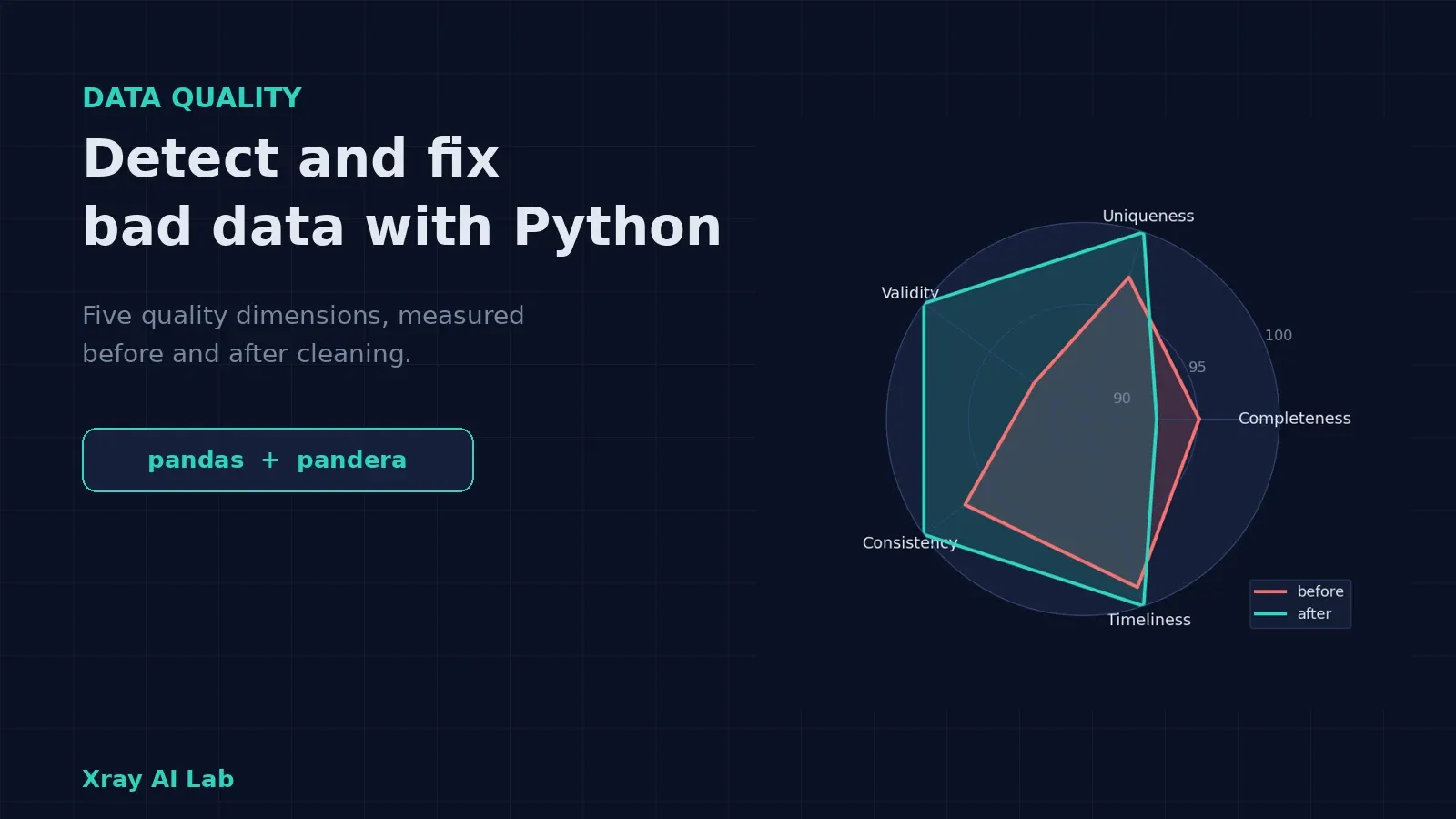
Data quality in data science means measuring how well a dataset fits its purpose, then detecting and fixing the cases where it does not. The practical way to do that in Python is to test the data the way you test code: define rules for each quality dimension, run them to produce numbers, fix what can be fixed safely, flag what cannot, and lock the rules into a schema so the same problems cannot silently return.

This article builds that workflow end to end. To make the results checkable, we plant known defects in a dataset, so we can compare what our checks find against what we know is there. We also run a small experiment to show what bad data does to a machine learning model, because “garbage in, garbage out” is easy to say and more useful when measured.

By the end you will be able to:

• Name six data quality dimensions and write a Python check for each.
• Build a reusable audit that returns counts, not impressions.
• Choose between fixing, flagging, and dropping a bad value.
• Write a pandera schema that acts as an executable data contract.
• Explain, with evidence, why some data problems damage models more than others.

If you want deeper treatment of two ingredients, see Data Cleaning with Python and Pandas and How to Handle Missing Values in Pandas. For a worked exploratory project, see Exploratory Data Analysis (EDA) with Python.

What data quality means: six dimensions

“Bad data” is vague. Data quality dimensions split it into questions you can test. Different frameworks use slightly different lists, but six come up repeatedly in practitioner guides: completeness, uniqueness, validity, consistency, timeliness, and accuracy.

Dimension	The question it asks	Typical Python check
Completeness	Is the data that should be present actually present?	df.isna().mean()
Uniqueness	Is each real-world entity recorded once?	df.duplicated(), df["id"].duplicated()
Validity	Do values obey type, format, and range rules?	pandera checks, regex, between()
Consistency	Do fields (or sources) agree with each other?	cross-column rules, e.g. ship date vs. order date
Timeliness	Is the data recent enough, and are dates plausible?	latest date, future-date check
Accuracy	Does the value match reality?	comparison with a trusted reference, spot checks

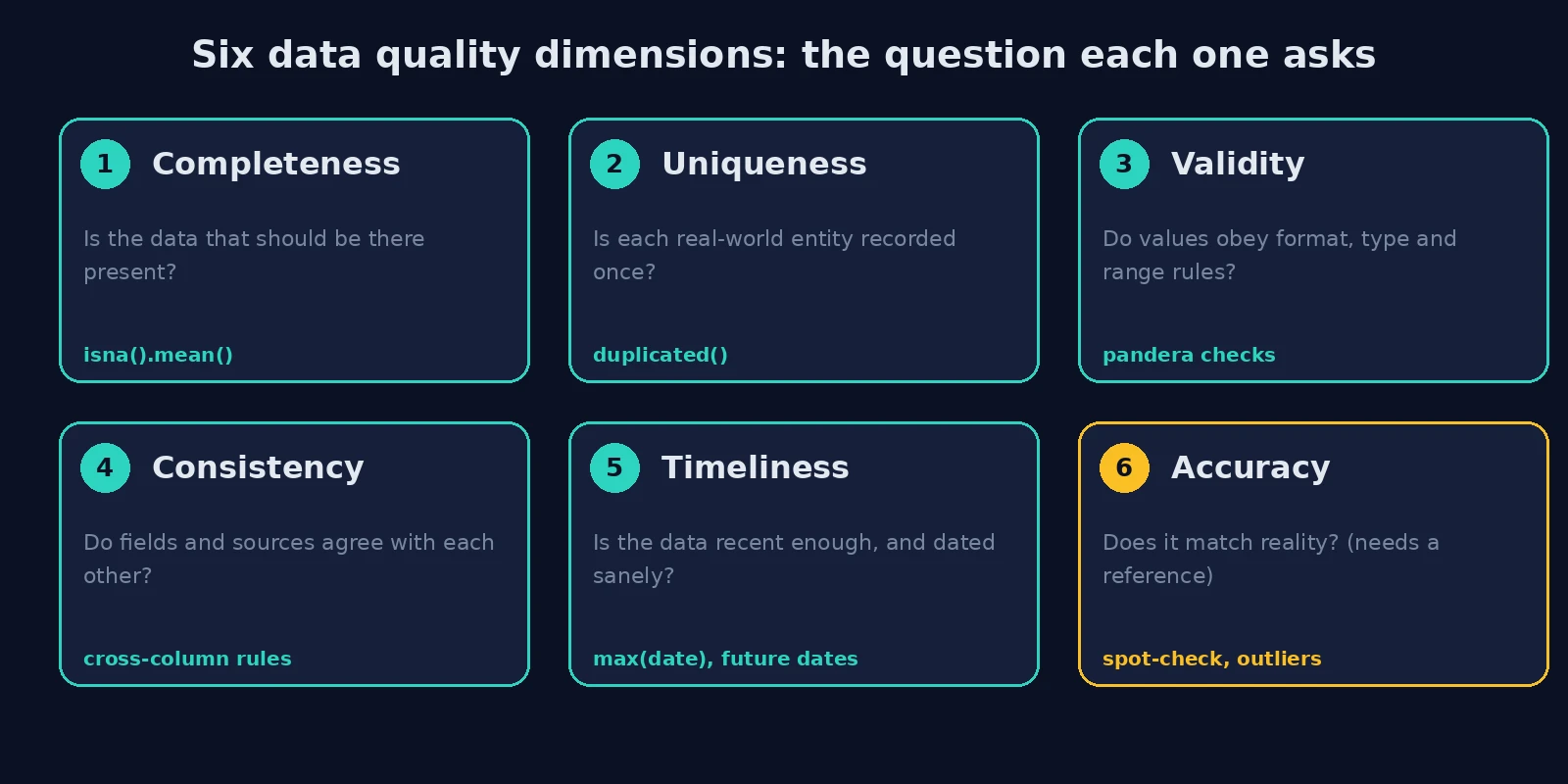
One honest caveat: accuracy cannot be fully tested from the data alone. If a customer’s recorded age is 34 and the true age is 43, no rule inside the table can know. You need a reference source or a manual check. What code can do is flag values that are suspicious, such as extreme outliers, and send them for review. The first five dimensions are testable by rules, and that is where automation pays off.

Why it matters: an experiment on model accuracy

Before building the workflow, let’s measure why it is worth the effort. I ran a small, reproducible experiment using the breast cancer dataset bundled with scikit-learn (569 samples, 30 numeric features). For each of 20 random seeds I trained a random forest and a single decision tree under four conditions:

1. Clean baseline: stratified 75/25 train/test split.
2. 10% label noise: 10% of training labels flipped; test labels left clean.
3. 20% label noise: the same with 20%.
4. Duplicate leakage: 50% of rows duplicated before a random split, so copies of the same record can land in both train and test.

import numpy as np, pandas as pd
from sklearn.datasets import load_breast_cancer
from sklearn.ensemble import RandomForestClassifier
from sklearn.tree import DecisionTreeClassifier
from sklearn.model_selection import train_test_split
from sklearn.metrics import accuracy_score

X, y = load_breast_cancer(return_X_y=True, as_frame=True)

def models(seed):
    return {"RandomForest": RandomForestClassifier(n_estimators=200, random_state=seed),
            "DecisionTree": DecisionTreeClassifier(random_state=seed)}

rows = []
for seed in range(20):
    rng = np.random.default_rng(seed)
    Xtr, Xte, ytr, yte = train_test_split(X, y, test_size=.25, stratify=y, random_state=seed)
    for name, m in models(seed).items():
        rows.append((name, "clean baseline", accuracy_score(yte, m.fit(Xtr, ytr).predict(Xte))))
    for p in (.10, .20):                                   # label noise on TRAIN only
        yn = ytr.copy(); flip = rng.choice(len(yn), int(p * len(yn)), replace=False)
        yn.iloc[flip] = 1 - yn.iloc[flip]
        for name, m in models(seed).items():
            rows.append((name, f"{int(p*100)}% label noise in training",
                         accuracy_score(yte, m.fit(Xtr, yn).predict(Xte))))
    dup = X.sample(frac=.5, random_state=seed)             # duplicates BEFORE the split
    Xd = pd.concat([X, dup]); yd = pd.concat([y, y.loc[dup.index]])
    Xtr2, Xte2, ytr2, yte2 = train_test_split(Xd, yd, test_size=.25, random_state=seed)
    for name, m in models(seed).items():
        rows.append((name, "50% duplicated rows before split",
                     accuracy_score(yte2, m.fit(Xtr2, ytr2).predict(Xte2))))

res = pd.DataFrame(rows, columns=["model", "scenario", "accuracy"])
print(res.groupby(["scenario", "model"])["accuracy"].agg(["mean", "std"]).mul(100).round(1)
         .unstack("model").to_string())

Results (test accuracy in %, mean over 20 seeds, standard deviation in the right-hand columns):

                                         mean                       std             
model                            DecisionTree RandomForest DecisionTree RandomForest
scenario                                                                            
10% label noise in training              84.0         95.7          3.5          2.0
20% label noise in training              73.5         93.8          3.7          2.4
50% duplicated rows before split         96.6         98.2          1.3          1.1
clean baseline                           93.0         96.3          3.0          1.5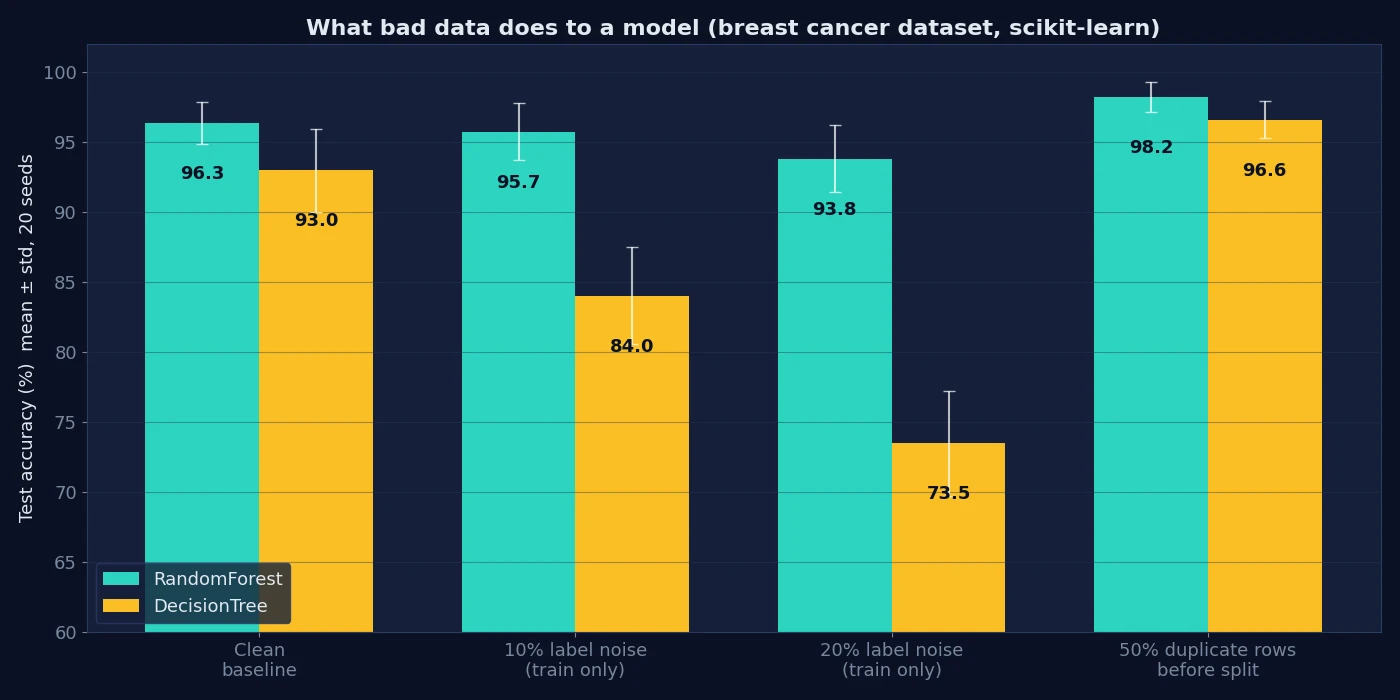

What this shows, and what it does not:

• Label noise hurts, but not equally. The single decision tree lost about 9 points at 10% noise and nearly 20 points at 20% noise. The random forest lost under 1 point and about 2.5 points. Averaging many trees makes ensembles more robust to noisy labels, but they still get worse.
• Duplicates make results look better, which is the dangerous direction. Accuracy rose from 93.0% to 96.6% (tree) and from 96.3% to 98.2% (forest), not because the models improved but because the test set contained copies of training rows. Bad data can inflate your evaluation and hide the problem until production.
• Limits of this experiment. It uses one clean, easy, well-studied dataset, and a single noise pattern (random label flips). The scenario 4 test sets are not identical to the baseline test sets, since the data was duplicated first. The y-axis in the chart starts at 60% to make differences visible. Treat the numbers as an illustration of direction, not a benchmark for other datasets.

The project: an orders table with planted defects

Real data does not come with an answer key. Ours will. The script below generates 500 synthetic orders, then deliberately plants eight kinds of defects in known quantities, then appends 15 duplicate rows. The data is synthetic, but the defect types are the ones that show up constantly in real order and customer tables.

import numpy as np, pandas as pd
import pandera.pandas as pa

AS_OF = pd.Timestamp("2026-10-24")      # the "today" the data is checked against
rng = np.random.default_rng(42)

n = 500
order_date = AS_OF - pd.to_timedelta(rng.integers(5, 400, n), unit="D")
df = pd.DataFrame({
    "order_id": np.arange(10_000, 10_000 + n),
    "customer_id": rng.integers(1, 200, n),
    "email": [f"user{i}@example.com" for i in rng.integers(1, 200, n)],
    "country": rng.choice(["MA", "FR", "ES", "US"], n, p=[.4, .25, .2, .15]),
    "order_date": order_date,
    "quantity": rng.integers(1, 6, n),
    "amount": rng.gamma(shape=4, scale=25, size=n).round(2),
})
df["ship_date"] = df["order_date"] + pd.to_timedelta(rng.integers(1, 8, n), unit="D")
df["email"] = df["email"].astype("object")

idx = rng.permutation(n)
cut = lambda a, b: idx[a:b]
planted = {}
df.loc[cut(0, 25), "amount"] = np.nan;                          planted["missing_amount"] = 25
df.loc[cut(25, 37), "amount"] = -df.loc[cut(25, 37), "amount"]; planted["negative_amount"] = 12
df.loc[cut(37, 45), "email"] = "not-an-email";                  planted["invalid_email"] = 8
df.loc[cut(45, 65), "country"] = rng.choice(["Morocco", "maroc", "MA ", "france"], 20)
planted["country_variants"] = 20
df.loc[cut(65, 75), "ship_date"] = df.loc[cut(65, 75), "order_date"] - pd.Timedelta(days=3)
planted["ship_before_order"] = 10
df.loc[cut(75, 81), "order_date"] = AS_OF + pd.Timedelta(days=30); planted["future_order_date"] = 6
df.loc[cut(81, 86), "amount"] = df.loc[cut(81, 86), "amount"] * 100; planted["extreme_amount"] = 5
dups = df.sample(15, random_state=1)
df = pd.concat([df, dups], ignore_index=True);                  planted["duplicate_rows"] = 15

The planted counts are: 25 missing amounts, 12 negative amounts, 8 invalid emails, 20 country-label variants, 10 shipping dates before the order date, 6 future order dates, 5 extreme amounts (multiplied by 100, like a misplaced decimal), and 15 duplicate rows.

Step 1: Detect, with one check per dimension

Wrap the checks in a single function that returns counts. A function (rather than ad hoc notebook cells) means you can run the identical audit again after cleaning.

STD_COUNTRIES = {"MA", "FR", "ES", "US"}
EMAIL = r"[^@\s]+@[^@\s]+\.[^@\s]+"

def audit(d):
    r = {}
    r["completeness: missing amount"] = int(d["amount"].isna().sum())
    r["uniqueness: duplicate rows"] = int(d.duplicated().sum())
    r["uniqueness: duplicate order_id"] = int(d["order_id"].duplicated().sum())
    r["validity: amount <= 0"] = int((d["amount"] <= 0).sum())
    r["validity: bad email"] = int((d["email"].notna() & ~d["email"].fillna("").str.fullmatch(EMAIL)).sum())
    r["validity: non-standard country"] = int((~d["country"].isin(STD_COUNTRIES)).sum())
    r["consistency: ship before order"] = int((d["ship_date"] < d["order_date"]).sum())
    r["timeliness: order date in future"] = int((d["order_date"] > AS_OF).sum())
    a = d["amount"].dropna(); a = a[a > 0]
    q1, q3 = a.quantile([.25, .75]); hi = q3 + 3 * (q3 - q1)
    r["accuracy (suspect): amount > Q3+3*IQR"] = int((d["amount"] > hi).sum())
    return pd.Series(r, name="count")

before = audit(df)

completeness: missing amount             25
uniqueness: duplicate rows               15
uniqueness: duplicate order_id           15
validity: amount <= 0                    12
validity: bad email                       9
validity: non-standard country           22
consistency: ship before order           16
timeliness: order date in future          6
accuracy (suspect): amount > Q3+3*IQR     5

Compare with what we planted. Five checks match the planted counts exactly (25, 15, 12, 6, and 5), and three do not, which is instructive rather than a failure:

• Bad email: 9 found vs. 8 planted. One of the 15 duplicated rows was a copy of a row with a planted bad email, so the defect now appears twice.
• Non-standard country: 22 vs. 20. Same reason: two duplicated rows copied a planted country variant.
• Ship before order: 16 vs. 10. The six rows where we moved order_date into the future also left ship_date untouched, so their ship date now precedes the order date. Defects interact, and a good audit surfaces consequences you did not intend.

Two other details are worth noting. Duplicate order_id values (15) match the duplicate rows (15), which tells us these are true copies rather than different orders sharing an ID. And the extreme-amount rule uses a wide fence, 3 × IQR beyond Q3, to flag only blatant cases, in the spirit of “flag, then investigate.”

Step 2: Fix, flag, or drop

Detecting is the easy half. For each problem, decide what is safe to do automatically:

Problem	Action	Why
Exact duplicate rows	Drop	A copy carries no new information
Inconsistent country labels	Fix with an explicit mapping	The intended value is unambiguous
Negative amounts	Set to missing	We cannot know the true value; abs() would invent one
Invalid emails	Set to missing	A wrong value is worse than an honest gap
Ship date before order date	Flag, blank the date	One of the two dates is wrong, and we don’t know which
Future-dated orders	Drop	An order cannot have happened after today
Extreme amounts	Flag for review	Could be a typo or a legitimate large order

fixed = df.copy()
fixed = fixed.drop_duplicates()
country_map = {"morocco": "MA", "maroc": "MA", "ma": "MA", "france": "FR"}
c = fixed["country"].str.strip()
fixed["country"] = c.str.lower().map(country_map).fillna(c.str.upper())
fixed.loc[fixed["amount"] <= 0, "amount"] = np.nan          # invalid -> missing, never silently abs()
fixed.loc[~fixed["email"].str.fullmatch(EMAIL), "email"] = pd.NA
bad_ship = fixed["ship_date"] < fixed["order_date"]
fixed["ship_date_suspect"] = bad_ship                         # flag, do not guess
fixed.loc[bad_ship, "ship_date"] = pd.NaT
fixed = fixed[fixed["order_date"] <= AS_OF].copy()            # future-dated orders cannot be real
a = fixed["amount"].dropna(); q1, q3 = a.quantile([.25, .75]); hi = q3 + 3 * (q3 - q1)
fixed["amount_suspect"] = fixed["amount"] > hi                # flag for review

after = audit(fixed)

completeness: missing amount             37
uniqueness: duplicate rows                0
uniqueness: duplicate order_id            0
validity: amount <= 0                     0
validity: bad email                       0
validity: non-standard country            0
consistency: ship before order            0
timeliness: order date in future          0
accuracy (suspect): amount > Q3+3*IQR     5

rows before/after: 515 -> 494

Rows dropped: 15 duplicates and 6 future-dated orders, so 515 becomes 494. Missing amounts rose from 25 to 37, which is exactly the 12 negative values we converted to missing. That is the right outcome, and the scorecard below shows why it looks like a “loss” even though the data became more truthful. The five suspicious amounts are still present, now flagged rather than deleted, because only a person with business context can say whether they are errors.

Step 3: Turn the rules into an executable contract with pandera

An audit function is a start, but a schema documents the rules once and enforces them everywhere. pandera lets you declare column types and checks on a DataFrame and validate against them. With lazy=True, it collects all failures instead of stopping at the first, as described in the lazy validation guide.

schema = pa.DataFrameSchema({
    "order_id": pa.Column(int, unique=True),
    "customer_id": pa.Column(int, pa.Check.gt(0)),
    "email": pa.Column(str, pa.Check.str_matches(r"^[^@\s]+@[^@\s]+\.[^@\s]+$"), nullable=True),
    "country": pa.Column(str, pa.Check.isin(sorted(STD_COUNTRIES))),
    "order_date": pa.Column("datetime64[ns]", pa.Check.le(AS_OF)),
    "ship_date": pa.Column("datetime64[ns]", nullable=True),
    "quantity": pa.Column(int, pa.Check.in_range(1, 100)),
    "amount": pa.Column(float, pa.Check.gt(0), nullable=True),
}, checks=pa.Check(lambda d: (d["ship_date"].isna()) | (d["ship_date"] >= d["order_date"]),
                   error="ship_date must not precede order_date"),
   strict=False)

try:
    schema.validate(df, lazy=True)
except pa.errors.SchemaErrors as e:
    print(e.failure_cases.groupby("check")["index"].nunique().to_string())

schema.validate(fixed, lazy=True)       # raises if anything is still wrong

check                                         distinct rows failing
field_uniqueness                              30
greater_than(0)                               12
isin(['ES', 'FR', 'MA', 'US'])                22
less_than_or_equal_to(2026-10-24 00:00:00)     6
ship_date must not precede order_date         16
str_matches('^[^@\s]+@[^@\s]+\.[^@\s]+$')      9

The raw table fails six checks and the cleaned table passes silently. Two details to interpret correctly. The uniqueness failure count of 30 is 15 pairs, because pandera reports every member of a duplicated group, not just the extra copy. And the numbers line up with the audit (12, 22, 6, 16, 9), which is a useful cross-check: two independent implementations of the same rules agree.

(I used pandera 0.34.1. Newer versions import via pandera.pandas, as shown; older tutorials import pandera directly.)

Step 4: Report a scorecard

Numbers make progress visible and make regressions obvious. Here is a simple percentage score per dimension, computed before and after:

def score(d):
    bad = (d["amount"] <= 0) | ~d["email"].fillna("x@y.z").str.fullmatch(EMAIL) | ~d["country"].isin(STD_COUNTRIES)
    return {
        "completeness (amount)": 1 - d["amount"].isna().mean(),
        "uniqueness (order_id)": 1 - d["order_id"].duplicated().mean(),
        "validity (amount>0, email, country)": 1 - bad.mean(),
        "consistency (ship>=order)": 1 - (d["ship_date"] < d["order_date"]).mean(),
        "timeliness (no future dates)": 1 - (d["order_date"] > AS_OF).mean(),
    }
sc = pd.DataFrame({"before": score(df), "after": score(fixed)}).mul(100).round(1)

                                     before  after
completeness (amount)                  95.1   92.5
uniqueness (order_id)                  97.1  100.0
validity (amount>0, email, country)    91.7  100.0
consistency (ship>=order)              96.9  100.0
timeliness (no future dates)           98.8  100.0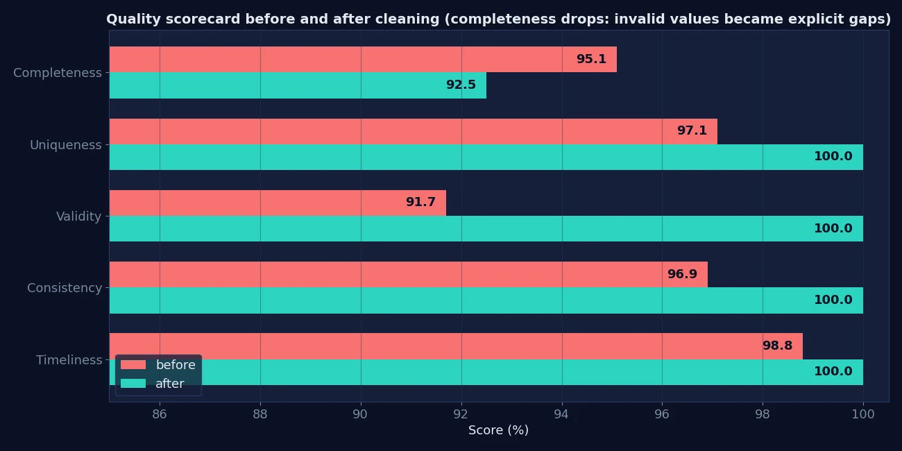

Completeness fell from 95.1% to 92.5%. That looks like cleaning made the data worse, but it didn’t: we replaced 12 impossible negative amounts with honest gaps. A completeness score can drop when validity rises, because you stopped counting wrong values as present. Scores are diagnostics, not goals to maximize in isolation. Choose targets per dimension and per column, based on the cost of an error.

From script to pipeline: make quality checks routine

A one-off cleanup decays. To keep quality from regressing:

• Validate at the boundary. Run the schema right after loading data and right before saving or training.
• Fail loudly on contract violations, and let softer metrics (such as the scorecard) feed monitoring and dashboards.
• Split before you deduplicate or engineer features. The duplicate-leakage experiment shows why: check uniqueness before a train/test split.
• Version the rules. A schema file in version control is documentation that cannot go stale.
• Log what you removed. Keep counts of dropped and flagged rows per run.
• Consider dedicated tooling as you scale. pandera suits DataFrame-centric workflows; Great Expectations is another open-source Python framework built around data quality expectations and dimensions.

Common mistakes

• Fixing without detecting. If you cannot count the problem before and after, you do not know you fixed it.
• “Repairing” values by guessing. Taking abs() of a negative amount, or filling a typo with the mean, invents data.
• Deduplicating after the split. Copies in both partitions inflate evaluation scores, as measured above.
• Treating all outliers as errors. Flag, review, and decide with domain knowledge.
• Optimizing a single score. Dimensions trade off, as completeness did here.
• Assuming rules are universal. Every threshold in this article (3 × IQR, the email pattern, the country list) is an assumption for this dataset.

Practice exercises

1. Add a check that flags orders whose quantity is outside 1 to 5 and see what the audit reports. (Answer: 0 for this dataset, because quantities were generated within 1 to 5.)
2. Using the audit output, how many rows differ between the raw and fixed tables, and why? (Answer: 21, which is 15 duplicates plus 6 future-dated orders.)
3. Why does the pandera uniqueness failure report 30 rather than 15? (Answer: it reports every member of each duplicated group, and 15 pairs give 30 rows.)

Conclusion

Data quality becomes manageable once it stops being a feeling and becomes a set of testable rules: define dimensions, measure them with a reusable audit, decide per defect whether to fix, flag, or drop, then encode the rules in a schema that fails loudly. In our experiment, the stakes were concrete. Label noise cut a single tree’s accuracy by up to roughly 20 points, and duplicates made evaluation look better than it should.

The logical next step is to apply this workflow to a real dataset of your own: write the audit first, look at the numbers, then decide what is safe to fix. Pair it with Data Cleaning with Python and Pandas for the cleaning mechanics.

Frequently asked questions

What are the dimensions of data quality?

Commonly cited dimensions include completeness, uniqueness, validity, consistency, timeliness, and accuracy. Frameworks vary a little, so pick the ones that match the decisions your data supports and define a testable rule for each.

How do I detect bad data in Python?

Write explicit checks per dimension: isna() for completeness, duplicated() for uniqueness, ranges, regexes and type checks for validity, and cross-column comparisons for consistency. Wrap them in a function so the same audit can be rerun after cleaning.

What is the difference between data cleaning and data validation?

Cleaning changes the data to fix problems; validation checks whether the data meets stated rules without changing it. Use validation (for example, a pandera schema) to prove cleaning worked and to catch problems in new data.

Should I delete or impute invalid values?

Neither automatically. If the true value is unambiguous (a known label variant), fix it. If it is unknowable, set it to missing and decide how to handle missingness later. Deleting rows loses information; guessing invents it.

Does bad data always reduce model accuracy?

No, and that is what makes it dangerous. In the experiment above, label noise reduced accuracy, but duplicate leakage raised measured accuracy while making the evaluation less trustworthy.

Is pandera or Great Expectations better?

They overlap. pandera is lightweight and fits DataFrame code; Great Expectations is a broader framework for expectation suites and data documentation. The best choice depends on your pipeline and team, so try both on a small dataset.

Can code guarantee accurate data?

No. Rules catch invalid, inconsistent, duplicated and implausible values, but accuracy needs a trusted reference or human review. Use outlier flags as a prompt to investigate, not as proof of error.