Exploratory Data Analysis (EDA) with Python: A Complete Project

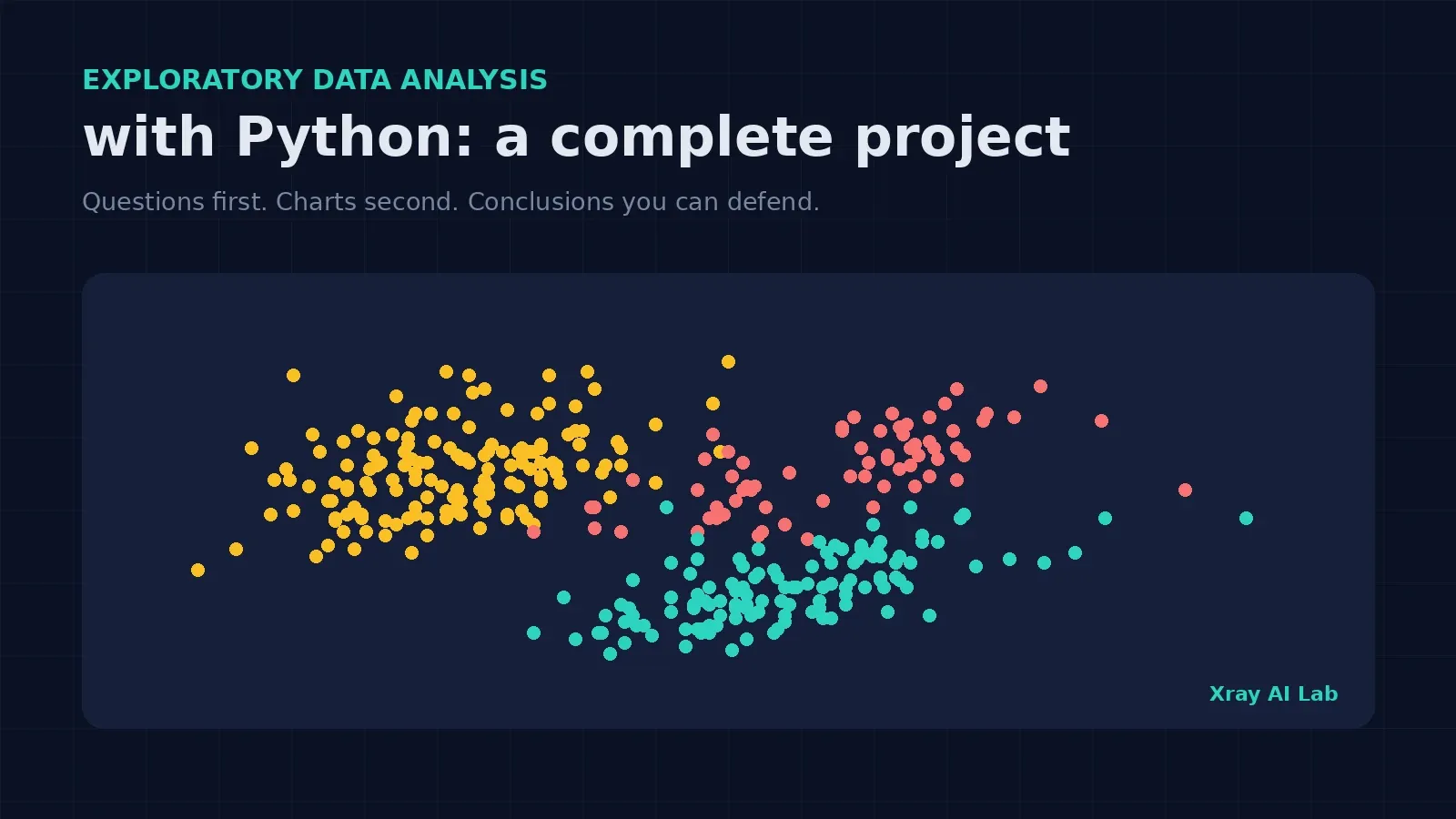
Exploratory data analysis (EDA) with Python is the process of questioning a dataset, using summary statistics and charts, before you clean it further, model it, or report on it. A good EDA does not end with a gallery of plots. It ends with answers, decisions, and a list of things that could mislead you later.

This article is a complete, runnable project. We will explore the Palmer Penguins dataset step by step, asking one question at a time: Is the data trustworthy? Where is it missing? What does each variable look like? How do groups differ? Which relationships are real? Along the way you will hit a classic trap, a correlation that reverses sign once you split the data by group, and you will see how to catch it.

By the end you will be able to:

• Follow a repeatable EDA sequence that works on most tabular datasets.
• Check data quality and missingness patterns, not just totals.
• Compare groups and spot confounding between categorical variables.
• Recognize Simpson’s paradox and explain it with evidence.
• Turn your findings into concrete decisions for the modeling stage.

If pandas is new to you, begin with Python for Data Science: A Beginner’s Guide. Cleaning is a separate job from exploring, and two companion articles cover it: Data Cleaning with Python and Pandas and How to Handle Missing Values in Pandas.

What EDA is, and what it is not

EDA is an investigative mindset: you look at the data to learn what questions are worth asking, and you check whether the data can support the questions you already have. It is not hypothesis testing, and it is not proof. Patterns you find are leads, not conclusions.

The most useful habit is to start from questions, not from plotting functions. Each step in this project maps a question to a technique:

Question	Technique	Pandas / seaborn tools
What is in this table?	Structure and type check	shape, dtypes, head()
What is missing, and is it random?	Missingness audit	isna().sum(), grouped missing rates
What does each variable look like?	Univariate summaries	describe(), skew(), histograms
How big is each group?	Category counts	value_counts(), crosstab()
How do groups differ?	Grouped statistics	groupby(), box plots
Which variables move together?	Correlation and scatter plots	corr(), regplot()
Is a pooled pattern hiding subgroups?	Stratified analysis	groupby() + corr()

The project dataset

We will use the Palmer Penguins data: size measurements for adult foraging Adélie, Chinstrap, and Gentoo penguins observed on islands near Palmer Station, Antarctica. The data were collected by Dr. Kristen Gorman and the Palmer Station Long Term Ecological Research (LTER) Program, packaged for data science by Allison Horst, Alison Hill, and Kristen Gorman, and released under a CC0 license. The original study is Gorman KB, Williams TD, Fraser WR (2014), Ecological Sexual Dimorphism and Environmental Variability within a Community of Antarctic Penguins (Genus Pygoscelis), PLoS ONE 9(3): e90081 (doi:10.1371/journal.pone.0090081). More documentation is available on the palmerpenguins project site.

Why not Titanic or the Iris data? Penguins give us real missing values, a mix of numeric and categorical columns, and a built-in subgroup structure, which makes it a better rehearsal for real projects. Here is the setup. The file below is the copy distributed with seaborn’s example datasets, so you need an internet connection (or download the CSV once and read it locally).

import pandas as pd
import seaborn as sns
import matplotlib.pyplot as plt

URL = "https://raw.githubusercontent.com/mwaskom/seaborn-data/master/penguins.csv"
df = pd.read_csv(URL)

All code in this article was executed with Python, pandas 3.0.2, and seaborn 0.13.2. Outputs shown are the real results of those runs.

Step 1: Check the structure of the data

Always begin with the basics: how many rows and columns, and what type is each?

print(df.shape)
print(df.dtypes.to_string())

(344, 7)
species                  str
island                   str
bill_length_mm        float64
bill_depth_mm         float64
flipper_length_mm     float64
body_mass_g           float64
sex                      str

We have 344 penguins and 7 columns: three categorical (species, island, sex) and four numeric measurements. Under pandas 3.0, text columns appear as str rather than object; on pandas 2.x you would see object here and everything below still works.

Also check for exact duplicate rows:

print("duplicated rows:", int(df.duplicated().sum()))   # 0

There are none, so there is nothing to remove at this stage.

Step 2: Audit missing values, including their pattern

Totals alone are not enough. You want to know where values are missing and whether the gaps cluster.

print(df.isna().sum().to_string())
print("rows with any missing:", int(df.isna().any(axis=1).sum()))

species               0
island                0
bill_length_mm        2
bill_depth_mm         2
flipper_length_mm     2
body_mass_g           2
sex                  11
rows with any missing: 11

Eleven rows have a gap, but the real story is in the pattern. The four measurement columns each miss exactly 2 values. Checking confirms that those are the same 2 rows (index 3 and 339), which have no measurements at all. The other 9 incomplete rows are missing only sex. Grouping the missing sex values by species gives:

print(df[df["sex"].isna()].groupby("species").size().to_string())

species
Adelie    6
Gentoo    5

No Chinstrap penguin is missing sex. In rates, that is about 3.9% of Adelie, 4.0% of Gentoo, and 0% of Chinstrap. With so few missing cases, this is probably not a serious problem, but it is exactly the kind of pattern you should note rather than hide. After dropping every incomplete row you would keep 333 complete cases (len(df.dropna())).

Decision for now: do not impute or drop anything yet. For each analysis below, pandas skips missing values automatically in describe(), mean() and corr(), and I explicitly drop missing sex only where sex is the grouping variable.

Step 3: Summarize each numeric variable

num = ["bill_length_mm", "bill_depth_mm", "flipper_length_mm", "body_mass_g"]
print(df[num].describe().round(1).to_string())
print(df[num].skew().round(2).to_string())

       bill_length_mm  bill_depth_mm  flipper_length_mm  body_mass_g
count           342.0          342.0              342.0        342.0
mean             43.9           17.2              200.9       4201.8
std               5.5            2.0               14.1        802.0
min              32.1           13.1              172.0       2700.0
25%              39.2           15.6              190.0       3550.0
50%              44.4           17.3              197.0       4050.0
75%              48.5           18.7              213.0       4750.0
max              59.6           21.5              231.0       6300.0

bill_length_mm       0.05
bill_depth_mm       -0.14
flipper_length_mm    0.35
body_mass_g          0.47

What can we conclude, and what can’t we?

• Plausible ranges. Body mass runs from 2,700 g to 6,300 g, and flipper length from 172 to 231 mm. Nothing is negative or absurd, so there are no obvious data-entry errors.
• No IQR outliers. I applied the 1.5 × IQR rule to each column across the whole dataset and found zero flagged values. That is reassuring, but a pooled summary can hide subgroup structure, as the next steps show.
• Mild skew. Skewness is small (at most 0.47, for body mass), so these variables are not heavily skewed, and a log transform is not obviously needed.
• A warning sign. The pooled mean bill length is 43.9 mm, and the standard deviation is 5.5 mm. Later we will see the species averages are 38.8, 48.8, and 47.5 mm. When a single variable is a blend of groups with different centers, the pooled mean describes none of them well.

Step 4: Count the categories and look for entanglement

print(df["species"].value_counts().to_string())
print(df["island"].value_counts().to_string())
print(pd.crosstab(df["species"], df["island"]).to_string())

species                      island
Adelie       152             Biscoe       168
Gentoo       124             Dream        124
Chinstrap     68             Torgersen     52

island      Biscoe  Dream  Torgersen
species                             
Adelie          44     56         52
Chinstrap        0     68          0
Gentoo         124      0          0

(The first two outputs are shown side by side for brevity.) The cross-tabulation is the first important finding: species and island are heavily entangled. Every Gentoo penguin was observed on Biscoe, every Chinstrap on Dream, and Torgersen has only Adélie penguins. Only Adélie penguins appear on all three islands.

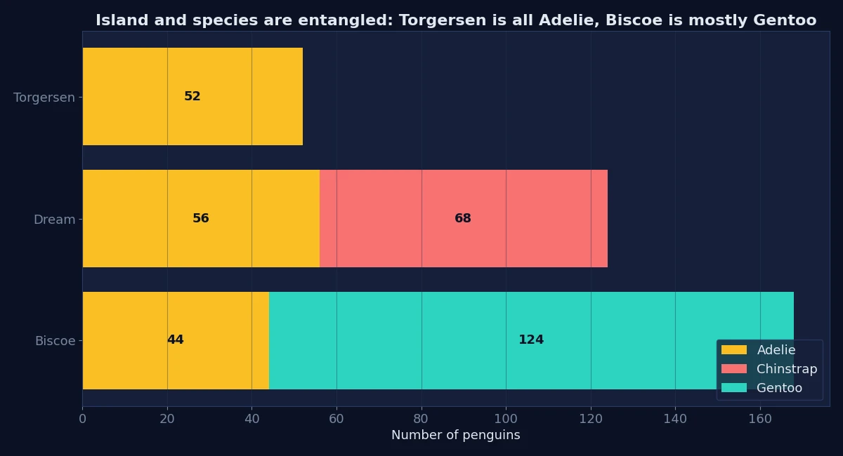
This matters later. If you compare islands without controlling for species, you are mostly comparing species. And if you try to predict species, the island column partly gives the answer away, so think carefully before including it as a feature.

Step 5: Compare groups

Now let’s quantify how species and sex differ.

print(df.groupby("species")[num].mean().round(1).to_string())
print(df.groupby(["species", "sex"])["body_mass_g"].mean().round(0).unstack().to_string())

           bill_length_mm  bill_depth_mm  flipper_length_mm  body_mass_g
species                                                                 
Adelie               38.8           18.3              190.0       3700.7
Chinstrap            48.8           18.4              195.8       3733.1
Gentoo               47.5           15.0              217.2       5076.0

sex        FEMALE    MALE
species                   
Adelie     3369.0  4043.0
Chinstrap  3527.0  3939.0
Gentoo     4680.0  5485.0

Three observations follow from the numbers:

1. Gentoo penguins are the heaviest, with a mean body mass of about 5,076 g against roughly 3,700 g for the other two species, and they have the longest flippers and the shallowest bills.
2. Adélie and Chinstrap are similar in body mass (3,701 vs 3,733 g), yet differ in bill length (38.8 vs 48.8 mm). Bill length separates them better than weight does.
3. Males are heavier than females in every species. The ratio of mean male to mean female mass is about 1.20 for Adélie, 1.12 for Chinstrap, and 1.17 for Gentoo. That is consistent with the sexual dimorphism studied in the original paper, though a ratio of means is a descriptive summary, not a statistical test.

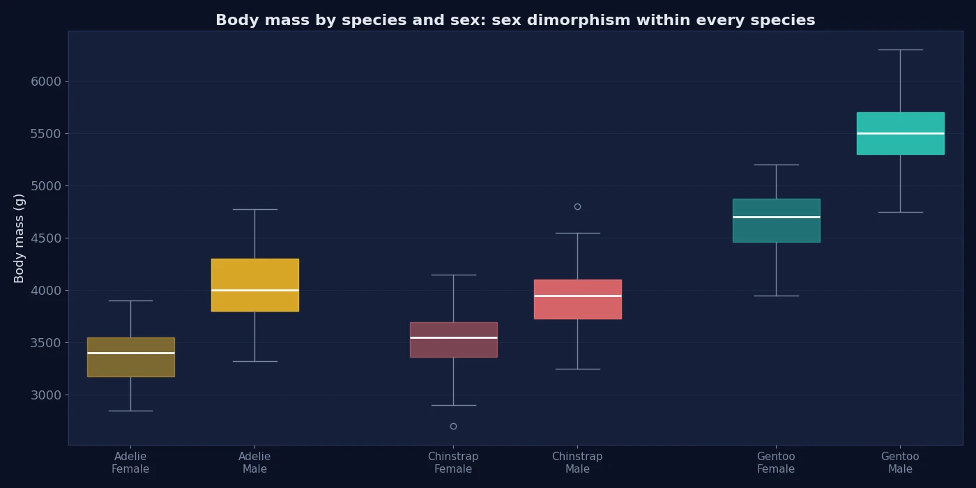
Box plots are the right chart here because they show the spread and overlap, not just the means. Notice how much the female and male boxes overlap within a species compared with the gap between Gentoo and the others.

Step 6: Examine relationships, and catch a trap

Start with the correlation matrix on the pooled data:

print(df[num].corr().round(2).to_string())

                   bill_length_mm  bill_depth_mm  flipper_length_mm  body_mass_g
bill_length_mm               1.00          -0.24               0.66         0.60
bill_depth_mm               -0.24           1.00              -0.58        -0.47
flipper_length_mm            0.66          -0.58               1.00         0.87
body_mass_g                  0.60          -0.47               0.87         1.00

A quick reading says that penguins with longer bills tend to have shallower bills (r = -0.24), and that flipper length and body mass are very strongly related (r = 0.87). The first conclusion is wrong, or at least badly misleading. Stratify by species and compare:

pooled = df["bill_length_mm"].corr(df["bill_depth_mm"])
within = df.groupby("species").apply(
    lambda g: g["bill_length_mm"].corr(g["bill_depth_mm"]), include_groups=False
)

pooled: -0.24
Adelie       0.39
Chinstrap    0.65
Gentoo       0.64

Within each species, longer bills go with deeper bills, with correlations of +0.39, +0.65, and +0.64. The pooled correlation is negative only because the species sit in different places on the chart: Gentoo have long, shallow bills, while Adélie have short, deep ones. This reversal is known as Simpson’s paradox: a trend in aggregated data that disappears or reverses when the data is split by a lurking grouping variable.

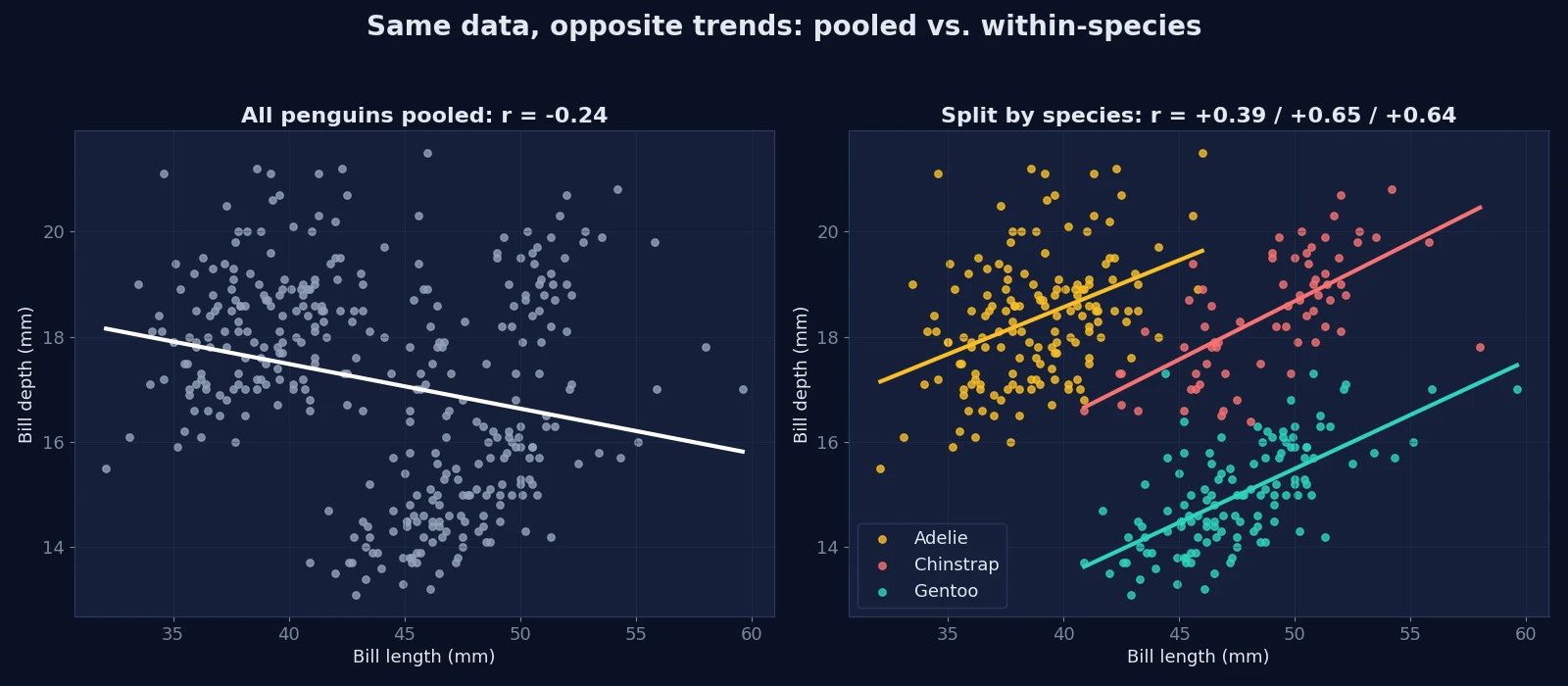
You can reproduce the pair of charts with a few lines of seaborn:

fig, axes = plt.subplots(1, 2, figsize=(12, 4.5))
sns.regplot(data=df, x="bill_length_mm", y="bill_depth_mm", ax=axes[0])
for name, g in df.groupby("species"):
    sns.regplot(data=g, x="bill_length_mm", y="bill_depth_mm", label=name, ax=axes[1])
axes[1].legend()

The same effect, in milder form, appears in the strongest relationship in the matrix. Flipper length and body mass correlate at 0.87 overall, but within species the correlations are lower: 0.47 (Adélie), 0.64 (Chinstrap), and 0.70 (Gentoo). Part of the pooled strength comes from species differences, not from penguin-to-penguin variation within a species. The relationship is still positive everywhere; it is simply weaker than the pooled number suggests.

The lesson: when a categorical variable divides your data into clusters, always compare pooled and within-group statistics before interpreting a correlation.

Step 7: Turn findings into decisions

An EDA is only useful if it changes what you do next. Here is what this one tells us, and the evidence behind each point.

Finding	Evidence	Decision
2 rows contain no measurements	Same two rows missing all four numeric columns	Exclude them from any numeric analysis
11 rows lack sex (Adélie and Gentoo only)	Grouped missing counts	Report it; test whether results change with and without them
Species and island are entangled	Cross-tabulation	Don’t interpret island effects without controlling for species; treat island as a leakage risk if species is the target
Bill length separates Adélie from Chinstrap better than mass	Group means	Keep it as a candidate predictor
Pooled correlations can mislead	Bill length vs depth reversed sign	Analyze within species, or include species as a variable
Males are heavier in every species	Group means and box plots	Include sex in any model of body mass; consider stratified splits

Notice what we did not do: we did not claim causes, run significance tests, or fit a model. These are descriptive findings from 344 observed penguins at one research site, so treat them as leads for the next stage, not final conclusions.

Common EDA mistakes

• Plotting before asking. Charts without a question produce trivia.
• Looking only at pooled summaries. Averages across groups can describe nobody.
• Treating missing totals as the whole story. Check which rows and which groups are affected.
• Reading correlation as causation. Correlation is a description, and confounders like species can reverse it.
• Ignoring categorical entanglement. Cross-tabulate your categorical columns before comparing them to anything.
• Letting outlier rules make decisions. Flag unusual values, then investigate.
• Not writing down decisions. An EDA that does not record what you will do differently is incomplete.

Practice exercises

1. How many penguins have complete records? Answer: 333 (len(df.dropna())).
2. Which species has no missing sex values? Answer: Chinstrap.
3. On which island(s) were Gentoo penguins observed? Answer: Biscoe only.
4. Without code, would you expect the pooled correlation between bill depth and body mass to be misleading? Compute the within-species values and check your answer. (Pooled is -0.47, and Gentoo are heavy with shallow bills, so there is reason to be suspicious.)

Conclusion

A complete EDA follows a pattern you can reuse: verify the structure, audit missingness, summarize variables, count categories, compare groups, inspect relationships, then record decisions. In this project the most valuable findings were not the prettiest charts. They were that species and island are entangled, that missing sex values cluster in two species, and that a pooled correlation can point in exactly the wrong direction.

A natural next step is to clean any remaining issues, then build a simple baseline model with a stratified train/test split, using what you learned here to choose features. If you want to strengthen the cleaning side first, read Data Cleaning with Python and Pandas.

Frequently asked questions

What are the main steps of exploratory data analysis in Python?

Check structure and types, audit missing values, summarize each variable, count categories, compare groups, examine relationships, and record the decisions your findings imply. Pandas covers most of the numeric work and seaborn or matplotlib covers the charts.

What is the difference between EDA and data cleaning?

EDA is about understanding the data and discovering problems; cleaning is about fixing them. In practice the two alternate: EDA reveals issues, cleaning resolves them, and a second look checks the result.

Which Python libraries do I need for EDA?

At minimum, pandas for summaries and grouping, plus matplotlib or seaborn for charts. NumPy is used underneath, and SciPy or statsmodels become useful when you move from description to formal testing.

How do I know if an outlier is an error?

You cannot tell from statistics alone. Check the raw record, the units, and whether the value is physically or logically possible. Flag it, investigate, and document what you decide.

What is Simpson’s paradox?

It is a situation where a trend visible in combined data reverses or disappears when the data is separated into groups. In this project, bill length and bill depth are negatively correlated overall but positively correlated within each species.

Should I drop rows with missing values during EDA?

Usually not at first. Study how much is missing and in which groups, then decide per analysis. Dropping rows too early can hide a pattern that matters.

Does EDA prove anything?

No. EDA generates questions and hypotheses; confirming them requires appropriate statistical testing or experiments, and causal claims need a suitable study design.