Gradient Descent Explained with Python: Math, Visualization, and Code

Gradient descent is how most machine learning models learn: it measures how wrong the model is with a loss function, computes which direction makes that loss grow fastest, and then steps the other way. Repeat that a few dozen or a few million times and the parameters settle near a minimum.

This article builds the method from scratch. You will derive the gradients for a linear model, implement gradient descent in about 15 lines of NumPy, and run a controlled experiment that shows exactly what the learning rate does, including the precise value above which training blows up. Every number in the results section comes from code that was actually run.

By the end you will be able to:

• Explain gradient descent in terms of loss, gradient, and step size.
• Derive the gradients of mean squared error (MSE) by hand and check them in code.
• Predict whether a learning rate will converge or diverge before running the training loop.
• Read a loss curve and a contour plot to diagnose what went wrong.

What gradient descent does, in plain terms

Imagine standing on a hilly surface in thick fog. You cannot see the lowest valley, but you can feel the slope under your feet. A sensible strategy is to take a step downhill, feel the slope again, and repeat.

Gradient descent is that strategy applied to a function $L(\theta)$, where $\theta$ is the vector of model parameters:

$$\theta_{t+1} = \theta_t - \eta \, \nabla L(\theta_t)$$

Symbol	Meaning
$\theta_t$	Parameters at iteration $t$
$L(\theta)$	Loss: a single number measuring how badly the model fits the data
$\nabla L(\theta)$	Gradient: the vector of partial derivatives, pointing toward steepest increase
$\eta$	Learning rate (step size), a positive hyperparameter you choose

The minus sign is the whole trick. The gradient points uphill, so we subtract it to go downhill. For a thorough survey of how this basic update is extended in practice (momentum, Adam, and others), see Sebastian Ruder’s An overview of gradient descent optimization algorithms.

The problem: fitting a line by minimizing MSE

We will use the simplest model that still has two parameters and a visible loss surface: a line $\hat{y} = wx + b$.

Step 1: define the loss

Given $n$ data points $(x_i, y_i)$, the mean squared error is

$$L(w, b) = \frac{1}{n} \sum_{i=1}^{n} \left( w x_i + b - y_i \right)^2$$

Squaring makes every error positive and penalizes large errors more than small ones. It also makes the loss a smooth bowl in $(w, b)$ space, which is what makes this problem a friendly place to learn.

Step 2: derive the gradients

Let the residual be $e_i = w x_i + b - y_i$. Applying the chain rule:

$$\frac{\partial L}{\partial w} = \frac{2}{n} \sum_{i=1}^{n} e_i \, x_i \qquad \frac{\partial L}{\partial b} = \frac{2}{n} \sum_{i=1}^{n} e_i$$

The update rules are therefore

$$w \leftarrow w - \eta \, \frac{\partial L}{\partial w}, \qquad b \leftarrow b - \eta \, \frac{\partial L}{\partial b}$$

Notice what the gradient is saying. If the model predicts too high on points with large positive $x$, the residuals $e_i$ are positive there, $\partial L / \partial w$ is positive, and the update lowers $w$. The math does what your intuition would.

Step 3: the curvature behind everything

For MSE the loss is a quadratic function of $(w, b)$, so its second derivatives (the Hessian) are constant:

$$H = \frac{2}{n} X^\top X, \qquad X = \begin{bmatrix} x_1 & 1 \\ \vdots & \vdots \\ x_n & 1 \end{bmatrix}$$

This matrix controls how fast and whether gradient descent converges. We will use it in a moment to predict the experiment’s outcome.

Implementing gradient descent in Python

The code below generates data from the line $y = 3x + 2$ plus Gaussian noise (standard deviation 1), implements the loss and gradients from the derivation, and runs gradient descent from a deliberately poor starting point, $(w, b) = (-4, -4)$.

import numpy as np

# Synthetic data: y = 3x + 2 + noise
rng = np.random.default_rng(42)
n = 100
x = rng.uniform(-3, 3, size=n)
y = 3.0 * x + 2.0 + rng.normal(0, 1.0, size=n)

def loss(w, b):
    return np.mean((w * x + b - y) ** 2)

def gradients(w, b):
    err = w * x + b - y                  # residuals e_i
    return 2 * np.mean(err * x), 2 * np.mean(err)

def gradient_descent(lr, steps=50, w0=-4.0, b0=-4.0):
    w, b = w0, b0
    path = [(w, b)]
    losses = [loss(w, b)]
    for _ in range(steps):
        gw, gb = gradients(w, b)
        w, b = w - lr * gw, b - lr * gb  # simultaneous update
        path.append((w, b))
        losses.append(loss(w, b))
    return np.array(path), np.array(losses)

Two details matter. First, both parameters are updated from gradients computed at the same point, not one after the other. Second, we record the full path and loss history, because a final number alone hides most of what is interesting.

Verify against a closed-form answer

Linear regression has an exact solution, which gives us a ground truth to check against. NumPy’s least-squares solver finds the loss minimum directly:

X = np.column_stack([x, np.ones(n)])
w_star, b_star = np.linalg.lstsq(X, y, rcond=None)[0]
L_star = loss(w_star, b_star)
print(f"Closed form: w={w_star:.4f}, b={b_star:.4f}, loss={L_star:.4f}")

Output from the executed script:

Closed form: w=3.0128, b=1.9870, loss=0.9589

The fitted values are close to the true $w = 3$ and $b = 2$ but not identical, because the noise in the sample shifts the optimum slightly. The minimum loss, 0.9589, is close to the noise variance of 1, which is what we expect from a well-specified model. Gradient descent should land on this same point.

Experiment: how the learning rate decides everything

We now run gradient descent for 50 iterations with five learning rates and compare against the closed-form optimum.

lrs = [0.005, 0.05, 0.1, 0.2, 0.4]
for lr in lrs:
    path, losses = gradient_descent(lr)
    print(f"lr={lr:<5} final w={path[-1,0]:.4f} b={path[-1,1]:.4f} loss={losses[-1]:.4f}")

Results

Learning rate	Final $w$	Final $b$	Final loss (50 steps)	Outcome
0.005	1.1039	−1.7533	23.5569	Stable but far too slow
0.05	3.0112	1.9538	0.9600	Converging, almost there
0.1	3.0128	1.9869	0.9589	Converged
0.2	3.0128	1.9870	0.9589	Converged, fastest of the five that converge
0.4	−5296.32	253.59	75,387,418	Diverged

The starting loss is 161.65 and the optimal loss is 0.9589. The table shows all three regimes: too small (0.005 barely moves), well tuned (0.1 and 0.2 reach the optimum), and too large (0.4 explodes).

To make “how fast” concrete, we also counted iterations until the loss was within $10^{-3}$ of the optimum:

Learning rate	Steps until loss − optimum < 0.001
0.05	51
0.1	24
0.2	11

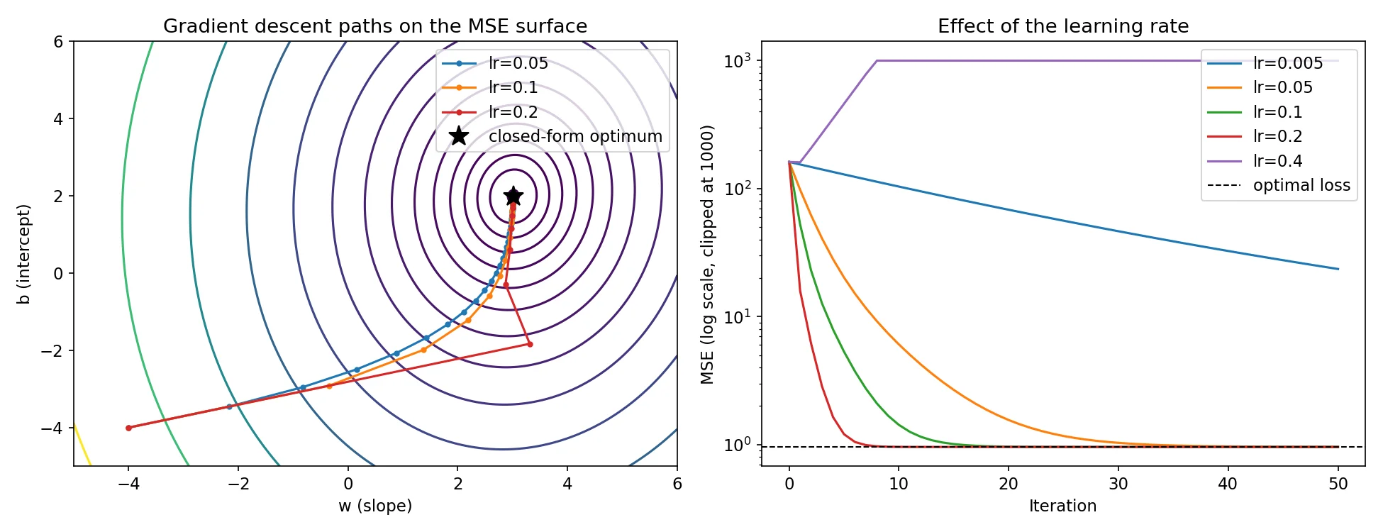
Left: paths on the loss surface. Right: loss versus iteration on a log scale (values clipped at 1000 so the diverging run fits on the chart).

Reading the plots

On the contour plot, each ring is a set of $(w, b)$ pairs with equal loss. The rings are elongated ellipses, not circles, and that shape explains the paths. The loss changes faster along one direction than the other, so the gradient does not point straight at the minimum. Early steps cut across the valley and later steps creep along it. The lr = 0.2 path even overshoots sideways on its first step before correcting.

On the loss curve, converging runs appear as nearly straight lines on a log axis, which means the error shrinks by a roughly constant factor each step. The lr = 0.005 curve is also a straight line, just with a very shallow slope.

Why 0.4 diverged: predicting convergence before training

The divergence at 0.4 is not bad luck. For a quadratic loss, the distance from the optimum $\theta^\*$ evolves exactly as

$$\theta_{t+1} - \theta^* = (I - \eta H)\,(\theta_t - \theta^*)$$

Break this into the eigenvectors of $H$. Along an eigenvector with eigenvalue $\lambda$, the error is multiplied by $(1 - \eta\lambda)$ every step. That factor must have magnitude below 1 for the error to shrink, which gives

$$0 < \eta < \frac{2}{\lambda_{\max}}$$

For our data, the Hessian eigenvalues (computed in the script with np.linalg.eigvalsh) are approximately 1.992 and 5.357. So the critical learning rate is

$$\frac{2}{5.357} \approx 0.373$$

That is why 0.2 converges and 0.4 diverges. Checking the per-step contraction factors $|1 - \eta\lambda|$ makes it concrete:

Learning rate	Factor along $\lambda = 1.992$	Factor along $\lambda = 5.357$	Slowest direction
0.005	0.990	0.973	0.990 (very slow)
0.05	0.900	0.732	0.900
0.1	0.801	0.464	0.801
0.2	0.602	0.071	0.602
0.4	0.203	1.143	1.143 (diverges)

At 0.4 the error along the steep direction grows by about 14% per step, so the loss, which depends on the squared error, grows by about $1.143^2 \approx 1.31$ per step. In the executed run, the loss in later iterations indeed rises by roughly 31% each step (for example, from 1337 to 1745 between steps 9 and 10).

The best fixed learning rate

Both directions matter. A small step is safe in the steep direction but slow in the shallow one. For a quadratic loss, the step size that minimizes the worst-case contraction factor is

$$\eta_{\text{opt}} = \frac{2}{\lambda_{\min} + \lambda_{\max}} \approx 0.272$$

The ratio $\kappa = \lambda_{\max} / \lambda_{\min} \approx 2.69$ is the condition number. The larger it is, the more elongated the contours and the slower gradient descent becomes, because the step size is capped by the steepest direction while progress in the flattest direction is throttled. This is one reason feature scaling matters in practice: it pushes the condition number toward 1.

Scope note. The exact $2/\lambda_{\max}$ threshold applies to quadratic losses like MSE on a linear model. For neural networks the loss is non-convex and the curvature changes from point to point, so the same idea gives a local guide, not an exact rule.

Choosing a stopping rule

The experiment used a fixed 50 iterations. Real training needs a stopping criterion, such as:

• Gradient norm below a tolerance: $\lVert \nabla L \rVert < \epsilon$ means the surface is nearly flat.
• Loss improvement below a tolerance: stop when the loss stops decreasing meaningfully.
• Maximum iterations: always keep this as a safety limit.
• Validation loss (for real models): stop when performance on held-out data stops improving, which guards against overfitting.

In our toy problem, every iteration used all 100 data points. That is batch gradient descent. For large datasets, stochastic and mini-batch variants compute the gradient from a subset of data per step, trading exactness for speed. Ruder’s overview, linked above, covers these variants in detail.

Common mistakes and how to diagnose them

Symptom	Likely cause	What to try
Loss grows or becomes inf/nan	Learning rate too large	Reduce $\eta$ by 2–10×; check input scaling
Loss decreases but extremely slowly	Learning rate too small, or ill-conditioned features	Increase $\eta$ cautiously; standardize features
Loss zig-zags and plateaus above the best value	Step too large near the minimum, or noisy gradients	Lower $\eta$ or use a decaying schedule
Parameters converge to different values than expected	Gradient formula bug	Compare against a numerical gradient (below)

Gradient checking

When you implement gradients by hand, verify them with finite differences:

def numerical_gradient(w, b, eps=1e-6):
    gw = (loss(w + eps, b) - loss(w - eps, b)) / (2 * eps)
    gb = (loss(w, b + eps) - loss(w, b - eps)) / (2 * eps)
    return gw, gb

print(gradients(-4.0, -4.0))
print(numerical_gradient(-4.0, -4.0))

In the executed run, the analytic gradient was approximately (−36.5590, −10.8563) and the numerical one matched to about eight decimal places. If your two outputs disagree, the bug is in your derivation or code, not in gradient descent. This is the cheapest way to catch a wrong minus sign.

Limitations of what we showed

• Convex, two-parameter problem. MSE on a line has one global minimum and no local minima or saddle points. Deep networks do not behave this cleanly.
• One dataset, one seed. Exact numbers such as “51 steps” depend on the data and starting point. The qualitative behavior (small is slow, large diverges, a threshold in between) generalizes; the specific values do not.
• Training loss only. We measured fit on the training data. We did not evaluate generalization to new data.
• Fixed learning rate. Practical optimizers adapt or schedule the step size.

Complete script

The following script reproduces every number and the figure in this article. It was run with Python 3, NumPy 2.4.4, and Matplotlib 3.10.8.

import numpy as np
import matplotlib.pyplot as plt

# 1. Synthetic data: y = 3x + 2 + noise
rng = np.random.default_rng(42)
n = 100
x = rng.uniform(-3, 3, size=n)
y = 3.0 * x + 2.0 + rng.normal(0, 1.0, size=n)

def loss(w, b):
    return np.mean((w * x + b - y) ** 2)

def gradients(w, b):
    err = w * x + b - y
    return 2 * np.mean(err * x), 2 * np.mean(err)

def gradient_descent(lr, steps=50, w0=-4.0, b0=-4.0):
    w, b = w0, b0
    path = [(w, b)]
    losses = [loss(w, b)]
    for _ in range(steps):
        gw, gb = gradients(w, b)
        w, b = w - lr * gw, b - lr * gb
        path.append((w, b))
        losses.append(loss(w, b))
    return np.array(path), np.array(losses)

# 2. Closed-form reference
X = np.column_stack([x, np.ones(n)])
w_star, b_star = np.linalg.lstsq(X, y, rcond=None)[0]
L_star = loss(w_star, b_star)
print(f"Closed form: w={w_star:.4f}, b={b_star:.4f}, loss={L_star:.4f}")

# Hessian and stability threshold: lr < 2 / lambda_max
H = 2 * (X.T @ X) / n
eig = np.linalg.eigvalsh(H)
print("Hessian eigenvalues:", np.round(eig, 4), "-> critical lr =", round(2 / eig.max(), 4))

# 3. Learning-rate experiment
lrs = [0.005, 0.05, 0.1, 0.2, 0.4]
results = {}
for lr in lrs:
    path, losses = gradient_descent(lr)
    results[lr] = (path, losses)
    print(f"lr={lr:<5} final w={path[-1,0]:.4f} b={path[-1,1]:.4f} loss={losses[-1]:.4f}")

for lr in [0.05, 0.1, 0.2]:
    _, losses = gradient_descent(lr, steps=500)
    hit = np.where(losses - L_star < 1e-3)[0]
    print(f"lr={lr}: steps to reach loss - L* < 1e-3: {hit[0] if len(hit) else 'not reached'}")

# 4. Plots
fig, axes = plt.subplots(1, 2, figsize=(13, 5))

ws = np.linspace(-5, 6, 200); bs = np.linspace(-5, 6, 200)
W, B = np.meshgrid(ws, bs)
Z = np.array([[loss(w, b) for w in ws] for b in bs])
axes[0].contour(W, B, Z, levels=np.logspace(-0.5, 2.3, 18), cmap="viridis")
for lr, c in zip([0.05, 0.1, 0.2], ["tab:blue", "tab:orange", "tab:red"]):
    p = results[lr][0]
    axes[0].plot(p[:, 0], p[:, 1], "o-", ms=3, color=c, label=f"lr={lr}")
axes[0].plot(w_star, b_star, "k*", ms=14, label="closed-form optimum")
axes[0].set_xlabel("w (slope)"); axes[0].set_ylabel("b (intercept)")
axes[0].set_title("Gradient descent paths on the MSE surface")
axes[0].legend()

for lr in lrs:
    axes[1].plot(np.clip(results[lr][1], None, 1e3), label=f"lr={lr}")
axes[1].axhline(L_star, color="k", ls="--", lw=1, label="optimal loss")
axes[1].set_yscale("log")
axes[1].set_xlabel("Iteration"); axes[1].set_ylabel("MSE (log scale, clipped at 1000)")
axes[1].set_title("Effect of the learning rate")
axes[1].legend()
plt.tight_layout()
plt.savefig("gradient-descent-learning-rate-experiment.png", dpi=150)

Install the dependencies with pip install numpy matplotlib if you do not already have them.

Exercises

1. Predict, then verify. Using $\eta_{\text{opt}} = 2/(\lambda_{\min}+\lambda_{\max})$, run gradient descent at that value. Does it reach the $10^{-3}$ threshold in fewer steps than 0.2? (Compute your prediction from the contraction factor first.)
2. Break the conditioning. Replace x with 100 * x and rerun. What happens to the critical learning rate? Then standardize x and compare.
3. Add a stopping rule. Modify gradient_descent to stop when the gradient norm falls below $10^{-4}$ and report the iteration count for each stable learning rate.

Conclusion

Gradient descent is a short loop: compute the loss gradient, step against it, repeat. What makes it work, or fail, is the relationship between the step size and the curvature of the loss. In our experiment, the Hessian predicted a critical learning rate near 0.373, and the runs agreed: 0.2 converged in 11 steps while 0.4 diverged. The same logic explains why unscaled features slow training, why loss curves look the way they do, and why optimizers such as momentum and Adam were invented.

Where to go next: try the exercises above, then move from this convex, two-parameter case to mini-batch training on a small neural network, where the loss surface is no longer a clean bowl. For a broader technical map of the optimizer family, read Ruder’s overview, and for the underlying calculus and numerical-computation background, the numerical computation chapter of Deep Learning by Goodfellow, Bengio, and Courville is a standard reference.

Frequently asked questions

What is gradient descent in simple terms?

It is an iterative method for minimizing a function. At each step you compute the gradient (the direction of steepest increase) and move a small distance in the opposite direction, repeating until the function stops decreasing.

What is the learning rate in gradient descent?

The learning rate $\eta$ is the multiplier that sets the step size. Too small and training is slow; too large and the updates overshoot and the loss can grow. For a quadratic loss, convergence requires $\eta < 2/\lambda_{\max}$, where $\lambda_{\max}$ is the largest eigenvalue of the Hessian.

How do I know when gradient descent has converged?

Common signs are a gradient norm close to zero, a loss that has stopped improving beyond a tolerance, or (when training real models) validation loss that has stopped improving. Always set a maximum number of iterations as well.

Does gradient descent always find the global minimum?

Only for convex problems such as MSE on a linear model, given a suitable learning rate. For non-convex problems such as neural networks, it can converge to local minima or stall near saddle points, and results can depend on initialization.

What is the difference between batch, stochastic, and mini-batch gradient descent?

Batch gradient descent computes the gradient from the full dataset each step. Stochastic gradient descent uses a single example, and mini-batch uses a small subset. Smaller batches are cheaper per step but give noisier gradient estimates.

Why does feature scaling help gradient descent?

Unscaled features make the loss surface elongated (a high condition number), so the largest safe step is limited by the steepest direction while progress in the flattest direction is slow. Standardizing features makes the contours rounder and speeds convergence.