Probability for Machine Learning: Bayes’ Theorem and Probability Distributions

A spam filter says an email is 97% likely to be spam. A classifier outputs 0.82 for “cat”. A regression model reports a prediction with an error bar. Each of these numbers is a statement about probability, and understanding where it comes from is what separates running a model from understanding it.

This guide covers the probability that matters most for machine learning: Bayes’ theorem and the probability distributions models are built from. You will work through numerical examples and check every one with Python. You will also see how probability explains common loss functions (cross-entropy and squared error) and why regularisation behaves the way it does.

Prerequisites are light: basic algebra and some Python. Every symbol is defined when it first appears.

Why Probability Matters in Machine Learning

Data is noisy, incomplete, and finite. Probability is the language for reasoning about that. In practice it shows up in three ways:

• Models predict probabilities. Logistic regression and neural network classifiers output a distribution over classes.
• Models assume distributions. Linear regression implicitly assumes errors follow a Gaussian (bell-curve) distribution.
• Training is estimation. Fitting parameters is often the same as finding the most probable parameters given the data.

Probability Basics You Need

Concept	Meaning	Example
Event	Something that may or may not happen	An email contains the word “free”
$P(A)$	Probability of event $A$, between 0 and 1	$P(\text{spam}) = 0.2$
$P(A \mid B)$	Probability of $A$ given that $B$ happened	$P(\text{spam} \mid \text{"free"})$
$P(A, B)$	Probability that both happen (joint)	Spam and contains “free”
Independence	Knowing $B$ does not change $P(A)$	$P(A, B) = P(A)\,P(B)$
Random variable	A number produced by a random process	Number of spam emails in a batch of 10

Two rules do most of the work. The product rule links joint and conditional probability:

$$P(A, B) = P(A \mid B)\,P(B)$$

The law of total probability adds up over every way $B$ can happen. If $A$ either happens or doesn’t:

$$P(B) = P(B \mid A)\,P(A) + P(B \mid \lnot A)\,P(\lnot A)$$

Here $\lnot A$ means “not $A$”.

Bayes’ Theorem

Where it comes from

The product rule can be written in two ways, because $P(A, B) = P(B, A)$:

$$P(A \mid B)\,P(B) = P(B \mid A)\,P(A)$$

Divide both sides by $P(B)$ and you have Bayes’ theorem:

$$P(H \mid D) = \frac{P(D \mid H)\,P(H)}{P(D)}$$

It is usually written with $H$ for a hypothesis and $D$ for observed data, and each piece has a name:

Term	Name	Question it answers
$P(H)$	Prior	What did I believe before seeing the data?
$P(D \mid H)$	Likelihood	How likely is this data if the hypothesis is true?
$P(D)$	Evidence	How likely is this data overall?
$P(H \mid D)$	Posterior	What should I believe after seeing the data?

The evidence is computed with the law of total probability, which is why the posterior always lands between 0 and 1.

Worked example: a spam filter

Suppose 20% of incoming email is spam, so $P(\text{spam}) = 0.2$. The word “free” appears in 60% of spam and in 5% of legitimate email (called “ham”). An email arrives containing “free”. How likely is it to be spam?

$$P(\text{spam} \mid \text{free}) = \frac{0.60 \times 0.20}{0.60 \times 0.20 + 0.05 \times 0.80} = \frac{0.12}{0.12 + 0.04} = 0.75$$

The numerator is spam emails containing “free”, and the denominator is all emails containing “free”. The same arithmetic is clearer with counts:

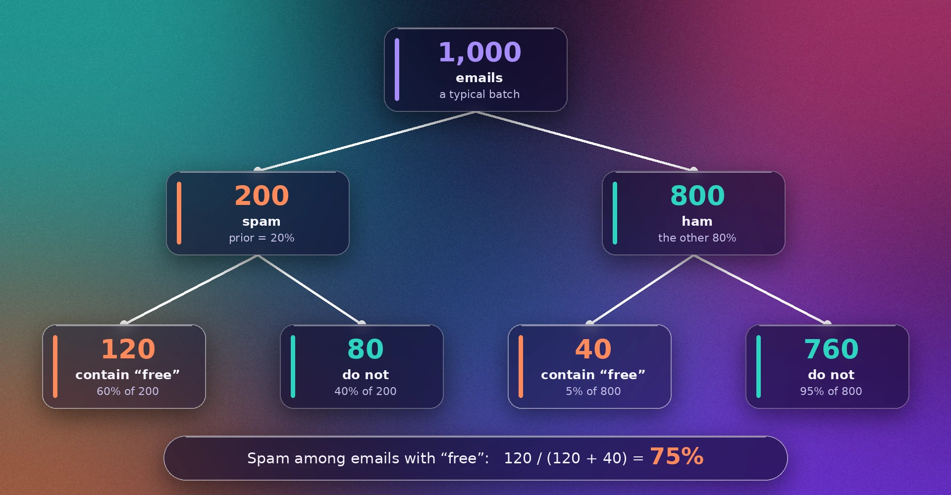
Of 1,000 emails, 120 spam and 40 ham contain “free”. Out of those 160, 120 are spam: 75%. Notice the result is far from the 60% you might guess from the likelihood alone. The prior matters, because spam is the minority class.

Updating with more evidence

Posteriors can become priors. Suppose the word “winner” appears in 30% of spam and 2% of ham. If we treat the two words as independent given the class, the posterior after “free” (0.75) becomes the prior for “winner”:

$$P(\text{spam} \mid \text{free, winner}) = \frac{0.30 \times 0.75}{0.30 \times 0.75 + 0.02 \times 0.25} = \frac{0.225}{0.230} \approx 0.978$$

That independence assumption is exactly the “naive” assumption in naive Bayes classifiers. It is rarely true, but it makes the model simple, fast, and often surprisingly competitive for text.

Probability Distributions

A probability distribution describes how likely each value of a random variable is.

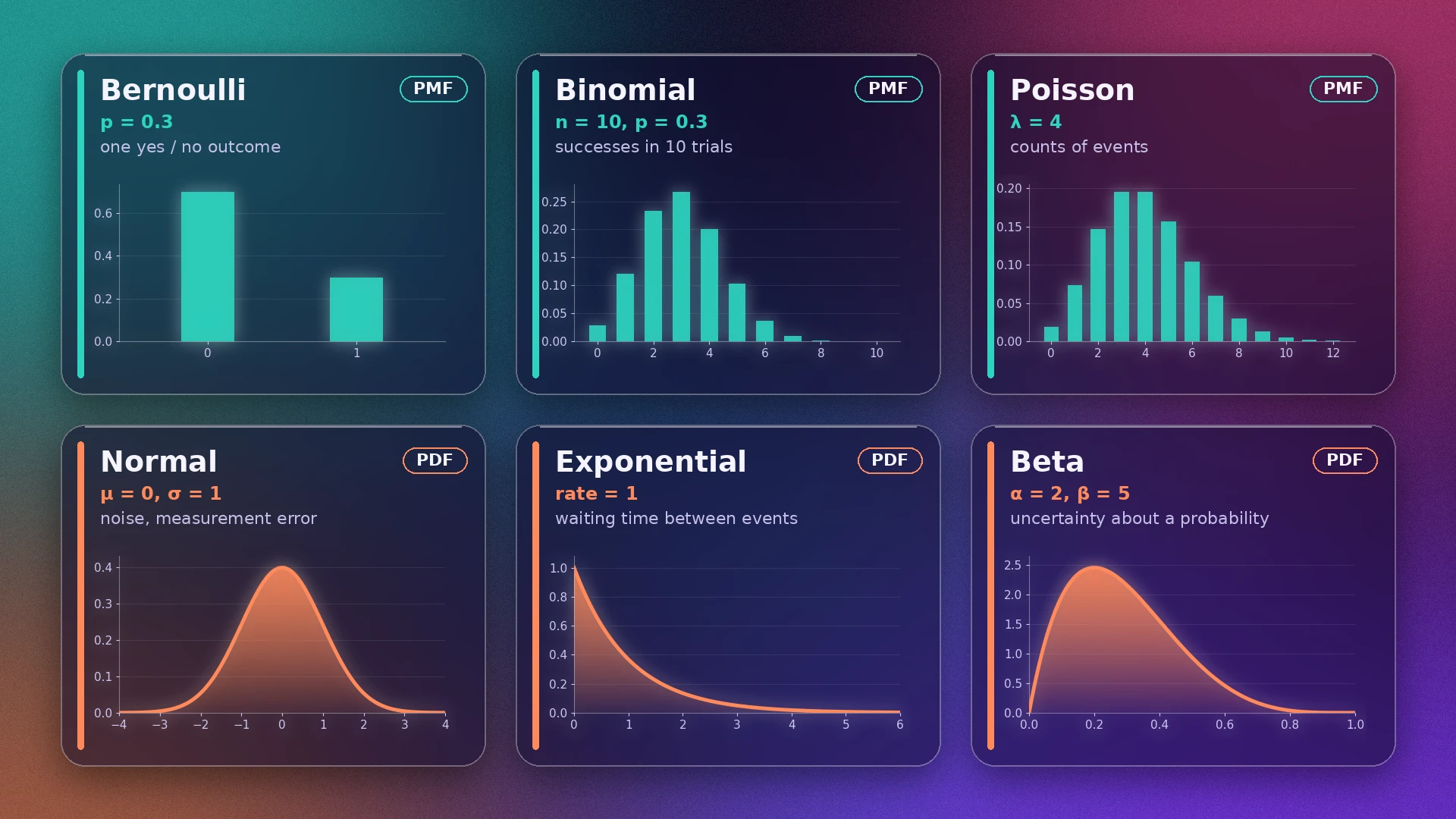
• A discrete variable takes separate values (0, 1, 2, …). Its distribution is a probability mass function (PMF), where each value has an actual probability.
• A continuous variable takes any value in a range. Its distribution is a probability density function (PDF). The probability of landing in an interval is the area under the curve, and the probability of any single exact value is zero.

The distributions you will meet most

Distribution	Type	Models	Typical ML use
Bernoulli($p$)	Discrete	One yes/no outcome	Binary labels, logistic regression output
Binomial($n$, $p$)	Discrete	Successes in $n$ trials	Click counts, A/B tests
Categorical	Discrete	One of $K$ classes	Softmax output of a classifier
Poisson($\lambda$)	Discrete	Counts of events per interval	Request counts, rare events
Normal($\mu$, $\sigma^2$)	Continuous	Symmetric noise around a mean	Regression errors, weight initialisation
Exponential($\lambda$)	Continuous	Waiting time between events	Time-to-event, survival models
Beta($\alpha$, $\beta$)	Continuous on [0, 1]	Uncertainty about a probability	Prior for click rates and success rates

The formulas for the most important ones:

$$\text{Bernoulli: } P(X = x) = p^{x}(1-p)^{1-x}, \quad x \in \{0, 1\}$$ $$\text{Binomial: } P(X = k) = \binom{n}{k} p^{k}(1-p)^{n-k}$$ $$\text{Normal: } f(x) = \frac{1}{\sigma\sqrt{2\pi}} \exp\!\left(-\frac{(x-\mu)^2}{2\sigma^2}\right)$$ $$\text{Beta: } f(p) = \frac{p^{\alpha-1}(1-p)^{\beta-1}}{B(\alpha, \beta)}$$

• $p$ is a success probability, $n$ is the number of trials, and $k$ the number of successes.
• $\mu$ is the mean and $\sigma^2$ the variance of the normal distribution.
• $B(\alpha, \beta)$ is a normalising constant that makes the Beta density integrate to 1.
• $\binom{n}{k}$ counts the ways to choose $k$ successes among $n$ trials.

Two facts trip up beginners. First, a PDF value is not a probability and can exceed 1: a Normal with standard deviation 0.1 has density 3.989 at its mean, because the curve is narrow and the total area is still 1. Second, the Normal distribution is common partly because sums of many small independent effects tend toward it (the central limit theorem), but real data is not always Gaussian.

Bayesian Estimation: A Click-Through Rate Example

Suppose an ad was shown 40 times and clicked 7 times. What is the true click-through rate?

The simple answer is $7/40 = 0.175$. That is the maximum likelihood estimate (MLE): the rate that makes the observed data most probable. But 40 impressions is a small sample, so we are uncertain, and Bayes’ theorem lets us quantify that.

We use a Beta prior for the unknown rate. Beta is conjugate to the Binomial likelihood, which means the posterior is also a Beta, with a simple update:

$$\text{Beta}(\alpha, \beta) \;\xrightarrow{\;k \text{ successes},\; n-k \text{ failures}\;}\; \text{Beta}(\alpha + k,\; \beta + n - k)$$

Starting with a mild Beta(2, 2) prior (a gentle belief that the rate is around 0.5) and 7 clicks in 40 impressions, the posterior is Beta(9, 35).

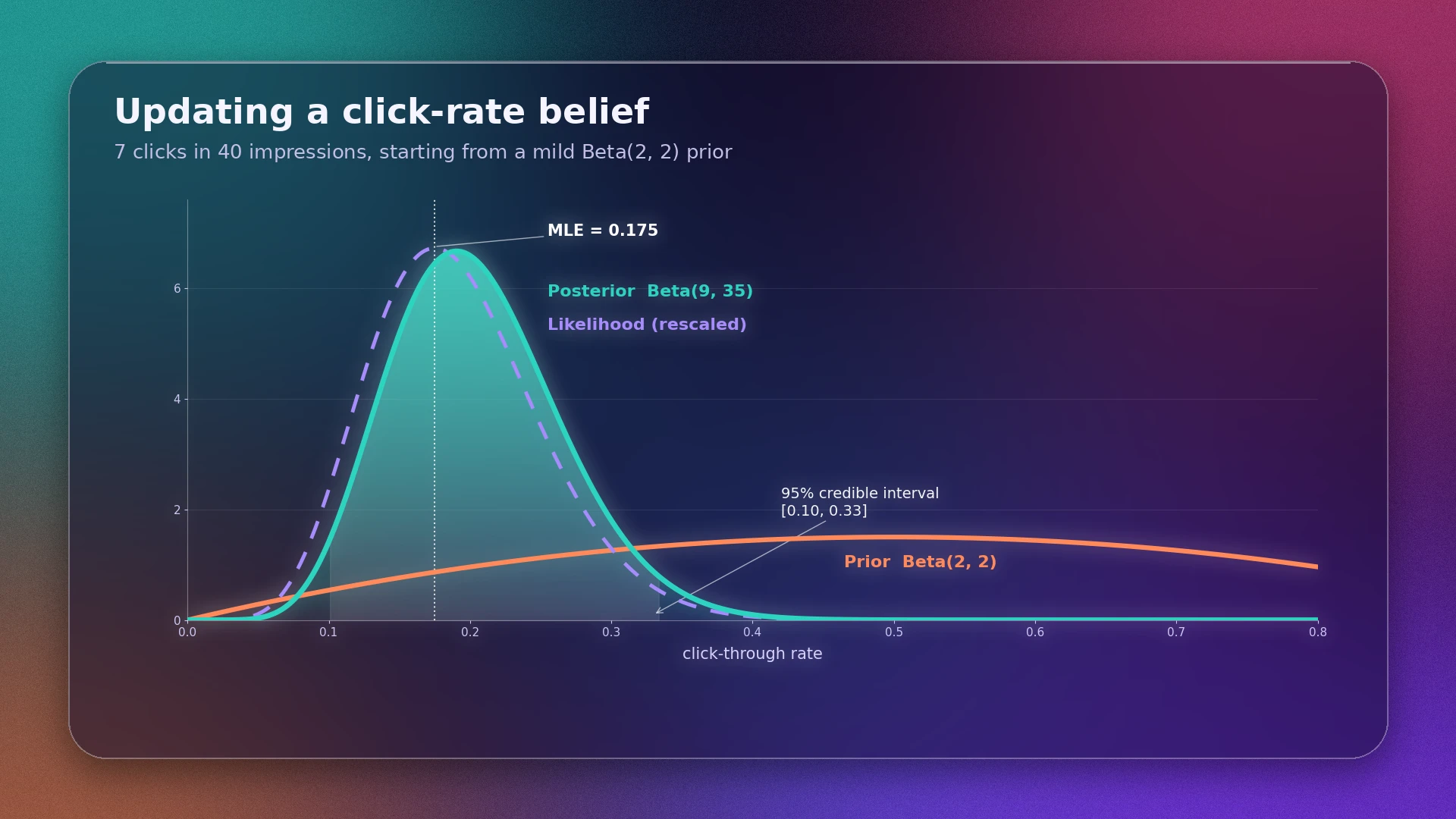
Three point estimates come out of this, and they differ for a reason:

• MLE = 0.175 ignores the prior entirely.
• MAP = 0.1905 is the posterior’s peak, $(\alpha - 1)/(\alpha + \beta - 2)$ for the posterior’s parameters.
• Posterior mean = 0.2045 averages over the whole posterior.

The prior pulls estimates slightly toward 0.5. With more data, the prior’s influence shrinks and all three converge. The 95% credible interval (the range containing 95% of the posterior probability) is [0.100, 0.334], which is wide and honest about how little 40 impressions tell us.

The same machinery compares variants. If variant B got 12 clicks in 45 impressions, sampling from both posteriors gives $P(\text{rate}_B > \text{rate}_A) \approx 0.82$. That is suggestive, not conclusive, and it depends on the prior and the small sample.

From Probability to Loss Functions

Many standard loss functions are negative log-likelihoods in disguise. Training by minimising them is the same as maximum likelihood estimation.

Model assumption	Negative log-likelihood becomes
Binary label ~ Bernoulli($p$)	Binary cross-entropy: $-\big[y\log p + (1-y)\log(1-p)\big]$
Class ~ Categorical (softmax)	Categorical cross-entropy: $-\log p_{\text{true class}}$
Target ~ Normal(prediction, $\sigma^2$), fixed $\sigma$	Squared error, up to a constant factor and offset

For the Gaussian case, the log-likelihood of one observation $y$ with prediction $\hat{y}$ is

$$\log f(y) = -\frac{(y-\hat{y})^2}{2\sigma^2} - \log\!\left(\sigma\sqrt{2\pi}\right)$$

Only the first term depends on the prediction, so maximising likelihood means minimising squared error.

Regularisation as a prior. Add a prior on the parameters and you get maximum a posteriori (MAP) estimation:

$$\hat{\theta}_{\text{MAP}} = \arg\max_{\theta}\; \big[\log P(D \mid \theta) + \log P(\theta)\big]$$

A Normal prior with mean 0 and standard deviation $\tau$ adds a term proportional to $\theta^2$, which is L2 regularisation (ridge). In the one-parameter example in the code below, with $n$ observations, noise standard deviation $\sigma$ and prior standard deviation $\tau$, the MAP estimate has a closed form:

$$\hat{\mu}_{\text{MAP}} = \frac{n\,\bar{y}}{n + \sigma^2/\tau^2}$$

Here $\bar{y}$ is the sample mean. The ratio $\sigma^2/\tau^2$ plays the role of the regularisation strength: a tighter prior (smaller $\tau$) shrinks the estimate harder toward 0.

Python: Check Every Number

The script below reproduces the spam posterior two ways (formula and a one-million-email simulation), compares distribution theory against samples, runs the click-through example, and confirms the MLE and MAP claims numerically.

Setup

pip install numpy scipy

The output below was produced with Python 3.12, NumPy 2.4.4 and SciPy 1.17.1. The random seed is fixed, so you should see the same numbers; other versions may differ in the last digits of simulated values.

The code

"""Probability for ML: Bayes' theorem, distributions, and Bayesian estimation, with checks."""
import numpy as np
from scipy import stats

rng = np.random.default_rng(42)

# ------------------------------------------------------------------
# 1. Bayes' theorem: does an email containing "free" look like spam?
# ------------------------------------------------------------------
def posterior(prior, lik_given_h, lik_given_not_h):
    """P(H | evidence) from a prior and two likelihoods."""
    evidence = lik_given_h * prior + lik_given_not_h * (1 - prior)  # law of total probability
    return lik_given_h * prior / evidence

p_spam = 0.20                                  # prior: P(spam)
p_free = {"spam": 0.60, "ham": 0.05}           # likelihoods: P("free" | class)
p_winner = {"spam": 0.30, "ham": 0.02}         # P("winner" | class)

after_free = posterior(p_spam, p_free["spam"], p_free["ham"])
after_both = posterior(after_free, p_winner["spam"], p_winner["ham"])  # yesterday's posterior is today's prior
print("--- Bayes' theorem ---")
print(f"P(spam | 'free')            = {after_free:.4f}")
print(f"P(spam | 'free' + 'winner') = {after_both:.4f}   (assumes words are independent given the class)")

# Monte Carlo check: simulate a million emails and count
n = 1_000_000
is_spam = rng.random(n) < p_spam
has_free = rng.random(n) < np.where(is_spam, p_free["spam"], p_free["ham"])
has_winner = rng.random(n) < np.where(is_spam, p_winner["spam"], p_winner["ham"])
print(f"simulated P(spam | 'free')            = {is_spam[has_free].mean():.4f}")
print(f"simulated P(spam | 'free' + 'winner') = {is_spam[has_free & has_winner].mean():.4f}")

# ------------------------------------------------------------------
# 2. Distributions: theory (scipy) vs. samples
# ------------------------------------------------------------------
print("\n--- Distributions: theory vs 200,000 samples ---")
dists = {
    "Bernoulli(p=0.3)":   stats.bernoulli(0.3),
    "Binomial(n=10,p=0.3)": stats.binom(10, 0.3),
    "Poisson(lam=4)":     stats.poisson(4),
    "Normal(mu=0,sd=1)":  stats.norm(0, 1),
    "Exponential(rate=1)": stats.expon(scale=1.0),
    "Beta(a=2,b=5)":      stats.beta(2, 5),
}
print(f"{'distribution':<22}{'mean':>8}{'var':>8}  {'sample mean':>12}{'sample var':>12}")
for name, d in dists.items():
    m, v = d.stats(moments="mv")
    x = d.rvs(size=200_000, random_state=rng)
    print(f"{name:<22}{float(m):>8.3f}{float(v):>8.3f}  {x.mean():>12.3f}{x.var():>12.3f}")

print(f"\nP(X = 3) for Binomial(10, 0.3): {stats.binom(10, 0.3).pmf(3):.4f}")
print(f"P(X = 2) for Poisson(4):        {stats.poisson(4).pmf(2):.4f}")
print(f"P(-1.96 < Z < 1.96), Normal:    {stats.norm.cdf(1.96) - stats.norm.cdf(-1.96):.4f}")
print(f"Normal(0, 0.1) density at 0:    {stats.norm(0, 0.1).pdf(0):.3f}   (a density can exceed 1)")

# ------------------------------------------------------------------
# 3. Beta-Binomial: estimating a click-through rate
# ------------------------------------------------------------------
a0, b0 = 2, 2                    # prior Beta(2, 2): mild belief that the rate is near 0.5
k, n_obs = 7, 40                 # 7 clicks in 40 impressions
a1, b1 = a0 + k, b0 + (n_obs - k)  # conjugate update: Beta(a + successes, b + failures)
post = stats.beta(a1, b1)

mle = k / n_obs
map_est = (a1 - 1) / (a1 + b1 - 2)   # mode of the posterior
lo, hi = post.ppf([0.025, 0.975])
print("\n--- Beta-Binomial: 7 clicks in 40 impressions ---")
print(f"posterior = Beta({a1}, {b1})")
print(f"MLE = {mle:.4f} | MAP = {map_est:.4f} | posterior mean = {post.mean():.4f}")
print(f"95% credible interval = [{lo:.3f}, {hi:.3f}]")

grid = np.linspace(0.001, 0.999, 99_901)
log_post = stats.binom.logpmf(k, n_obs, grid) + stats.beta.logpdf(grid, a0, b0)
print(f"grid-search MAP check   = {grid[log_post.argmax()]:.4f}")

# Compare two ad variants: A = 7/40, B = 12/45, same prior
pa = stats.beta(a0 + 7, b0 + 33).rvs(200_000, random_state=rng)
pb = stats.beta(a0 + 12, b0 + 33).rvs(200_000, random_state=rng)
print(f"P(rate_B > rate_A) = {(pb > pa).mean():.3f}")

# ------------------------------------------------------------------
# 4. Likelihood, loss functions and priors
# ------------------------------------------------------------------
print("\n--- Gaussian likelihood = squared error; Gaussian prior = L2 shrinkage ---")
y = rng.normal(5.0, 2.0, size=30)
mu = np.linspace(0, 10, 100_001)
sigma, tau = 2.0, 1.0            # noise sd and prior sd (prior mean 0)
sse = ((y[:, None] - mu[None, :]) ** 2).sum(axis=0)
nll = sse / (2 * sigma**2)                       # negative log-likelihood (constants dropped)
nlp = nll + mu**2 / (2 * tau**2)                 # add the negative log Gaussian prior
print(f"sample mean              = {y.mean():.4f}")
print(f"argmin squared error     = {mu[sse.argmin()]:.4f}")
print(f"argmin NLL (MLE)         = {mu[nll.argmin()]:.4f}")
print(f"argmin NLL + prior (MAP) = {mu[nlp.argmin()]:.4f}")
print(f"closed form MAP          = {len(y) * y.mean() / (len(y) + sigma**2 / tau**2):.4f}")

Output

--- Bayes' theorem ---
P(spam | 'free')            = 0.7500
P(spam | 'free' + 'winner') = 0.9783   (assumes words are independent given the class)
simulated P(spam | 'free')            = 0.7496
simulated P(spam | 'free' + 'winner') = 0.9785

--- Distributions: theory vs 200,000 samples ---
distribution              mean     var   sample mean  sample var
Bernoulli(p=0.3)         0.300   0.210         0.301       0.210
Binomial(n=10,p=0.3)     3.000   2.100         2.996       2.101
Poisson(lam=4)           4.000   4.000         4.001       4.017
Normal(mu=0,sd=1)        0.000   1.000        -0.001       0.996
Exponential(rate=1)      1.000   1.000         0.999       0.999
Beta(a=2,b=5)            0.286   0.026         0.285       0.026

P(X = 3) for Binomial(10, 0.3): 0.2668
P(X = 2) for Poisson(4):        0.1465
P(-1.96 < Z < 1.96), Normal:    0.9500
Normal(0, 0.1) density at 0:    3.989   (a density can exceed 1)

--- Beta-Binomial: 7 clicks in 40 impressions ---
posterior = Beta(9, 35)
MLE = 0.1750 | MAP = 0.1905 | posterior mean = 0.2045
95% credible interval = [0.100, 0.334]
grid-search MAP check   = 0.1905
P(rate_B > rate_A) = 0.822

--- Gaussian likelihood = squared error; Gaussian prior = L2 shrinkage ---
sample mean              = 5.4045
argmin squared error     = 5.4045
argmin NLL (MLE)         = 5.4045
argmin NLL + prior (MAP) = 4.7686
closed form MAP          = 4.7686

Reading the output

• Bayes: the formula and the simulation agree (0.7500 vs 0.7496, and 0.9783 vs 0.9785). The small gap is simulation noise.
• Distributions: sample means and variances match the theoretical values from scipy.stats, which confirms the parameter conventions. Note that SciPy’s exponential distribution uses scale = 1/rate.
• Click-through rate: the grid search finds the same MAP (0.1905) as the closed form, a useful check that the posterior formula is right.
• Loss functions: minimising squared error and minimising the Gaussian negative log-likelihood give the same answer (5.4045, the sample mean). Adding the prior moves the estimate to 4.7686, matching the closed form.

These checks cover the arithmetic in this article. They do not make the modelling assumptions true for your own data, such as independent words or Gaussian noise.

Common Mistakes

• Confusing $P(A \mid B)$ with $P(B \mid A)$. “Spam contains ‘free’ 60% of the time” is not “emails with ‘free’ are 60% spam”. The answer here was 75%, and a different prior would change it.
• Ignoring the base rate. A rare event with a good test can still yield mostly false alarms.
• Treating a density as a probability. Only areas under a PDF are probabilities.
• Assuming independence without checking. Naive Bayes works despite violated independence in many text tasks, but its probabilities are often poorly calibrated.
• Zero counts. If a word never appears in spam in training, its likelihood is 0 and a single occurrence forces the posterior to 0. Add smoothing, such as Laplace smoothing, which adds a small count to every category.
• Multiplying many small probabilities. Products underflow to 0. Work with log-probabilities and add instead.
• Reading a credible interval as a confidence interval. They answer different questions and come from different frameworks.
• Assuming a “flat” prior is neutral. Every prior is a modelling choice, including the flat one.

Limitations and Trade-Offs

• Priors are subjective. Different reasonable priors give different posteriors, especially with little data.
• Conjugate pairs are a convenience. Beta-Binomial has a closed form. Most real models do not, and need sampling or approximation methods.
• Distribution choices are assumptions. A Poisson model assumes the variance equals the mean, which many real count datasets violate.
• Good loss functions are not the whole story. A model can minimise cross-entropy and still produce poorly calibrated probabilities.

Practice Exercises

1. A medical test. A disease affects 1% of people. A test detects it 90% of the time, and gives a false positive for 5% of healthy people. If someone tests positive, what is the probability they have the disease?

2. Binomial. Each email is spam with probability 0.2, independently. What is the probability that exactly 2 of 5 emails are spam?

3. Beta update. Start with a uniform prior, Beta(1, 1). You observe 3 successes and 1 failure. What are the posterior, its mean, and its MAP estimate?

Solutions

1. $P(\text{disease} \mid +) = \dfrac{0.90 \times 0.01}{0.90 \times 0.01 + 0.05 \times 0.99} = \dfrac{0.009}{0.0585} \approx 0.154$. Even after a positive result, the chance is about 15%, because the disease is rare.
2. $\binom{5}{2}(0.2)^2(0.8)^3 = 10 \times 0.04 \times 0.512 = 0.2048$.
3. The posterior is Beta(4, 2). The mean is $4/6 \approx 0.667$ and the MAP is $(4-1)/(4+2-2) = 0.75$.

Frequently Asked Questions

What is Bayes’ theorem in one sentence?

It tells you how to update the probability of a hypothesis after seeing evidence: the posterior is proportional to the prior times the likelihood.

What is the difference between probability and likelihood?

Probability treats the parameters as fixed and asks how likely different data are. Likelihood treats the observed data as fixed and asks how plausible different parameter values are. They use the same formula, viewed from opposite directions.

What is the difference between a PMF and a PDF?

A PMF gives the probability of each discrete value. A PDF describes a continuous variable, and probabilities come from areas under it, not from its height.

Why is the Gaussian distribution used so often?

Partly because sums of many independent small effects tend to look Gaussian, and partly because it is mathematically convenient: its log-likelihood leads to squared error, which is easy to optimise. It is a modelling choice, not a law of nature.

Is cross-entropy loss related to probability?

Yes. For classification, cross-entropy is the negative log-likelihood of the true labels under the model’s predicted probabilities, so minimising it is maximum likelihood estimation.

Do I need Bayesian methods to do machine learning?

No. Many successful models use only maximum likelihood. Bayesian thinking helps most when data is scarce, when you have real prior knowledge, or when you need honest uncertainty estimates.

Next Steps

Re-run the script and change one number at a time. Raise the prior’s strength and watch the posterior stay put. Increase the impressions to 4,000 with the same 17.5% rate and watch the credible interval shrink and MLE and MAP converge. Then move on to maximum likelihood for logistic regression, and to Bayesian linear regression, where the weights themselves get distributions.

References

• Murphy, K. P. Probabilistic Machine Learning: An Introduction. MIT Press, 2022. A draft is freely available at probml.github.io/pml-book.
• Deisenroth, M. P., Faisal, A. A., and Ong, C. S. Mathematics for Machine Learning. Cambridge University Press, 2020. mml-book.com.
• Bishop, C. M. Pattern Recognition and Machine Learning. Springer, 2006.
• SciPy documentation, scipy.stats.